Introduction to Control Systems
Sources:
- Norman S. Nise. (2014). Chapter 1. Introduction. Control Systems Engineering (7th ed., pp. 1-21). WILEY.
Introduction to Control Systems
According to Wikipedia, control system manages, commands, directs, or regulates the behavior of other devices or systems using control loops.
Fundamentally, there are two types of control loop: open-loop control (feedforward), and closed-loop control (feedback).
In this article, we discuss two major configurations of control systems: open loop and closed loop. Open-loop systems do not monitor or correct the output for disturbances; however, they are simpler and less expensive than closed-loop systems.

Open-loop systems
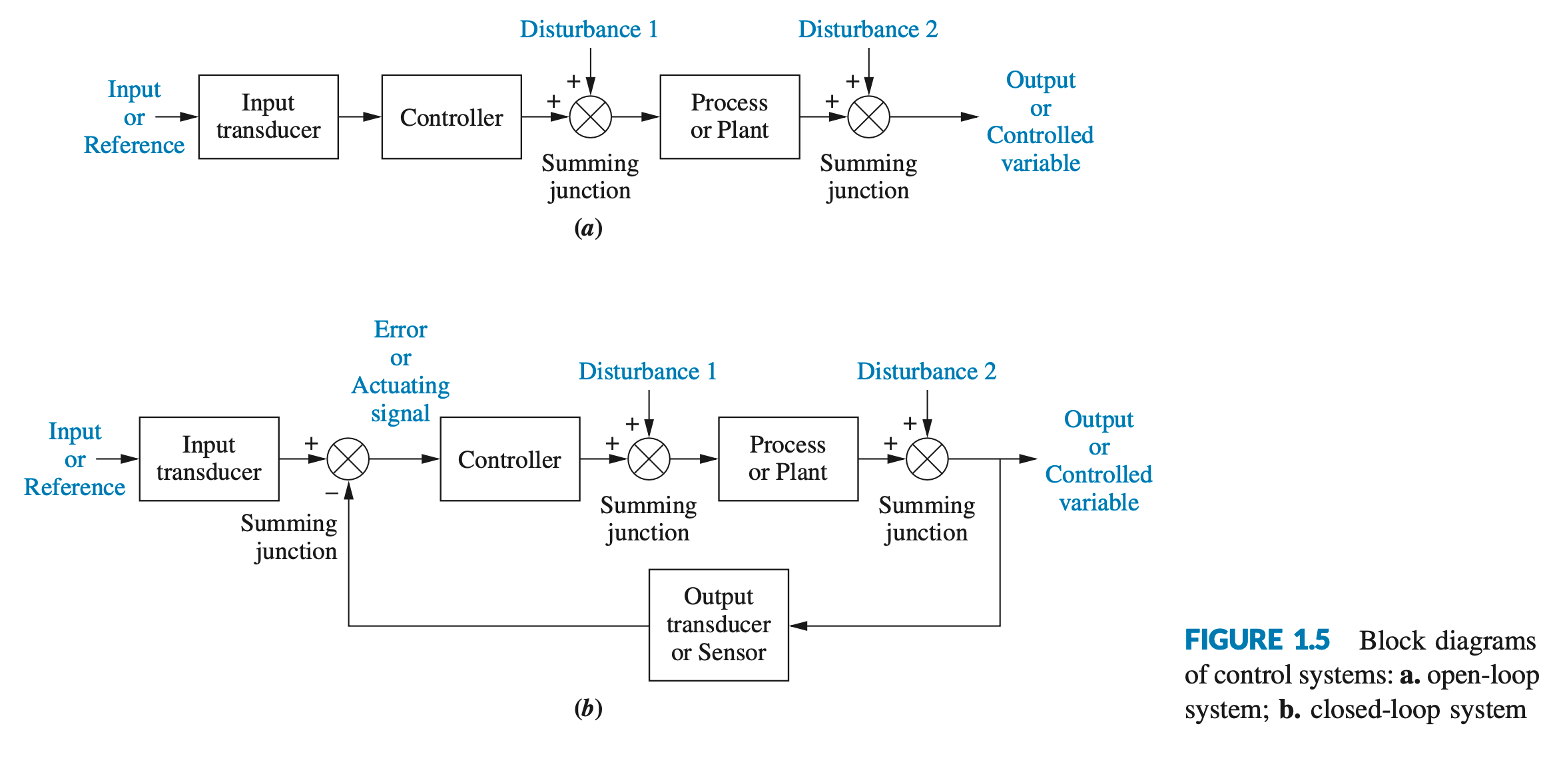
A generic open-loop system is shown in Figure 1.5(a).
- It starts with a subsystem called an input transducer, which converts the form of the input to that used by the controller.
- The controller drives a process or a plant.
- The input of the control system is sometimes called the reference, while the output can be called the controlled variable.
- Other signals, such as disturbances, are shown added to the controller and process outputs via summing junctions, which yield the algebraic sum of their input signals using associated signs. For example, the plant can be a furnace or air conditioning system, where the output variable is temperature. The controller in a heating system consists of fuel valves and the electrical system that operates the valves.
Drawbacks
An open-loop system has three drawbacks:
- It cannot compensate for any disturbances that add to the controller’s driving signal (Disturbance 1 in Figure 1.5(a)).
- It's output is corrupted not only by signals that add to the controller’s commands but also by disturbances at the output (Disturbance 2 in Figure 1.5(a)).
- The system cannot correct for these disturbances, either.
Closed-loop systems
The disadvantages of open-loop systems, namely sensitivity to disturbances and inability to correct for these disturbances, may be overcome in closed-loop systems. The generic architecture of a closed-loop system is shown in Figure 1.5(b).
- The input transducer converts the form of the input to the form used by the controller.
- An output transducer, or sensor, measures the output response and converts it into the form used by the controller. For example, if the controller uses electrical signals to operate the valves of a temperature control system, the input position and the output temperature are converted to electrical signals.
- The first summing junction algebraically adds the signal from the input to the signal from the output, which arrives via the feedback path, the return path from the output to the summing junction.
- In Figure 1.5(b), the output signal is subtracted from the input signal. The result is generally called the actuating signal. However, in systems where both the input and output transducers have unity gain (that is, the transducer amplifies its input by 1), the actuating signal’s value is equal to the actual difference between the input and the output. Under this condition, the actuating signal is called the error.
Closed-loop systems, then, have the obvious advantage of greater accuracy than open-loop systems. They are less sensitive to noise, disturbances, and changes in the environment. Transient response and steady-state error can be controlled more conveniently and with greater flexibility in closed-loop systems, often by a simple adjustment of gain (amplification) in the loop and sometimes by redesigning the controller. We refer to the redesign as compensating the system and to the resulting hardware as a compensator.
Mathematical models
Differential equation
Many systems can be approximately described by an equation called linear, time-invariant differential equation which relates the output, \(c(t)\), to the input, \(r(t)\), by way of the system parameters, \(a_i\) and \(b_j\). \[ \begin{equation} \label{eq_1_2} a_n \frac{d^n c(t)}{d t^n}+a_{n-1} \frac{d^{n-1} c(t)}{d t^{n-1}}+\cdots+a_0 c(t)=b_m \frac{d^m r(t)}{d t^m}+b_{m-1} \frac{d^{m-1} r(t)}{d t^{m-1}}+\cdots+b_0 r(t) \end{equation} \]
Note: The input, \(r(t)\), stands for reference input. The output, \(c(t)\), stands for controlled variable.
Transfer function
Although the differential equation relates the system to its input and output, it is not a satisfying representation from a system perspective. Looking at \(\eqref{eq_1_2}\), a general, \(n\) th-order, linear, time-invariant differential equation, we see that the system parameters, which are the coefficients, appear throughout the equation. In addition, the output, \(c(t)\), and the input, \(r(t)\), also appear throughout the equation.
We would prefer a mathematical representation such as that shown in Figure 2.1(a), where the input, output, and system are distinct and separate parts.

Also, we would like to represent conveniently the interconnection of several subsystems. For example, we would like to represent cascaded interconnections, as shown in Figure 2.1(b), where a mathematical function, called a transfer function, is inside each block, and block functions.
A transfer function is derived from the linear, time-invariant differential equation using what we call the Laplace transform.
Taking the Laplace transform of both sides of \(\eqref{eq_1_2}\), \[ \begin{aligned} & a_n s^n C(s)+a_{n-1} s^{n-1} C(s)+\cdots+a_0 C(s)+\text { initial condition terms involving } c(t) \\ = & b_m s^m R(s)+b_{m-1} s^{m-1} R(s)+\cdots+b_0 R(s)+\text { initial condition terms involving } r(t) \end{aligned} \] If we assume that all initial conditions are zero, this reduces to
\[ \left(a_n s^n+a_{n-1} s^{n-1}+\cdots+a_0\right) C(s)=\left(b_m s^m+b_{m-1} s^{m-1}+\cdots+b_0\right) R(s) \] Now form the ratio of the output transform, \(C(s)\), divided by the input transform, \(R(s)\): \[ \frac{C(s)}{R(s)}=G(s)=\frac{\left(b_m s^m+b_{m-1} s^{m-1}+\cdots+b_0\right)}{\left(a_n s^n+a_{n-1} s^{n-1}+\cdots+a_0\right)} \] Notice that Eq. (2.53) separates the output, \(C(s)\), the input, \(R(s)\), and the system, which is the ratio of polynomials in \(s\) on the right. We call this ratio, \(G(s)\), the transfer function and evaluate it with zero initial conditions.
State space model
Still another model is the state-space representation. One advantage of state-space methods is that they can also be used for systems that cannot be described by linear differential equations.