Value Iteration and Policy Iteration
- Shiyu Zhao. Chapter 4: Value Iteration and Policy Iteration. Mathematical Foundations of Reinforcement Learning.
- –> Youtube: Value Iteration and Policy Iteration
This chapter introduces three algorithms that are closely related to each other. Briefly speaking, they are all solutions of Bellman optimality equations (BOEs) to get optimal policies.
Value iteration
This section introduces the value iteration algorithm. It is exactly the algorithm suggested in solving the Bellman optimality equation (BOE). (This section is exactly the same of that chapter, there’s nothing new added here.)
The algorithm is \[ \begin{equation} \label{eq_solution_of_BOE} v_{k+1}=\max _{\pi \in \Pi}\left(\color{teal} {r_\pi} + \gamma \color{salmon} {P_\pi v_k} \right), \end{equation} \]
where \(k=0,1,2, \ldots\).
It is guaranteed that \(v_k\) and \(\pi_k\) converge to the optimal state value and an optimal policy as \(k \rightarrow \infty\), respectively.
But \(\eqref{eq_solution_of_BOE}\) can’t be calculated directly. In fact, value iteration is an iterative algorithm. Each iteration has two steps.
Step 1: policy update. This step is to solve \[ \begin{equation} \label{eq_policy_update} \pi_{k+1}=\arg \max _\pi\left(\color{teal} {r_\pi} + \gamma \color{salmon} {P_\pi v_k} \right) \end{equation} \] where \(v_k\) is obtained in the previous iteration.
Step 2: value update. It calculates a new value \(v_{k+1}\) by \[ \begin{equation} \label{eq_value_update} v_{k+1}=\color{teal}{r_{\pi_{k+1}}}+\gamma \color{salmon} {P_{\pi_{k+1}} v_k}, \end{equation} \] where \(v_{k+1}\) will be used in the next iteration.
Note: \(v_k\) is not a state value, it doesn’t ensure to satisfy the Bellman equation/
The value iteration algorithm introduced above is in a matrix-vector form. It’s useful for understanding the core idea of the algorithm.
To implement this algorithm, we need to further examine its elementwise form.
Elementwise form and implementation
Step 1
Step 1: Policy update
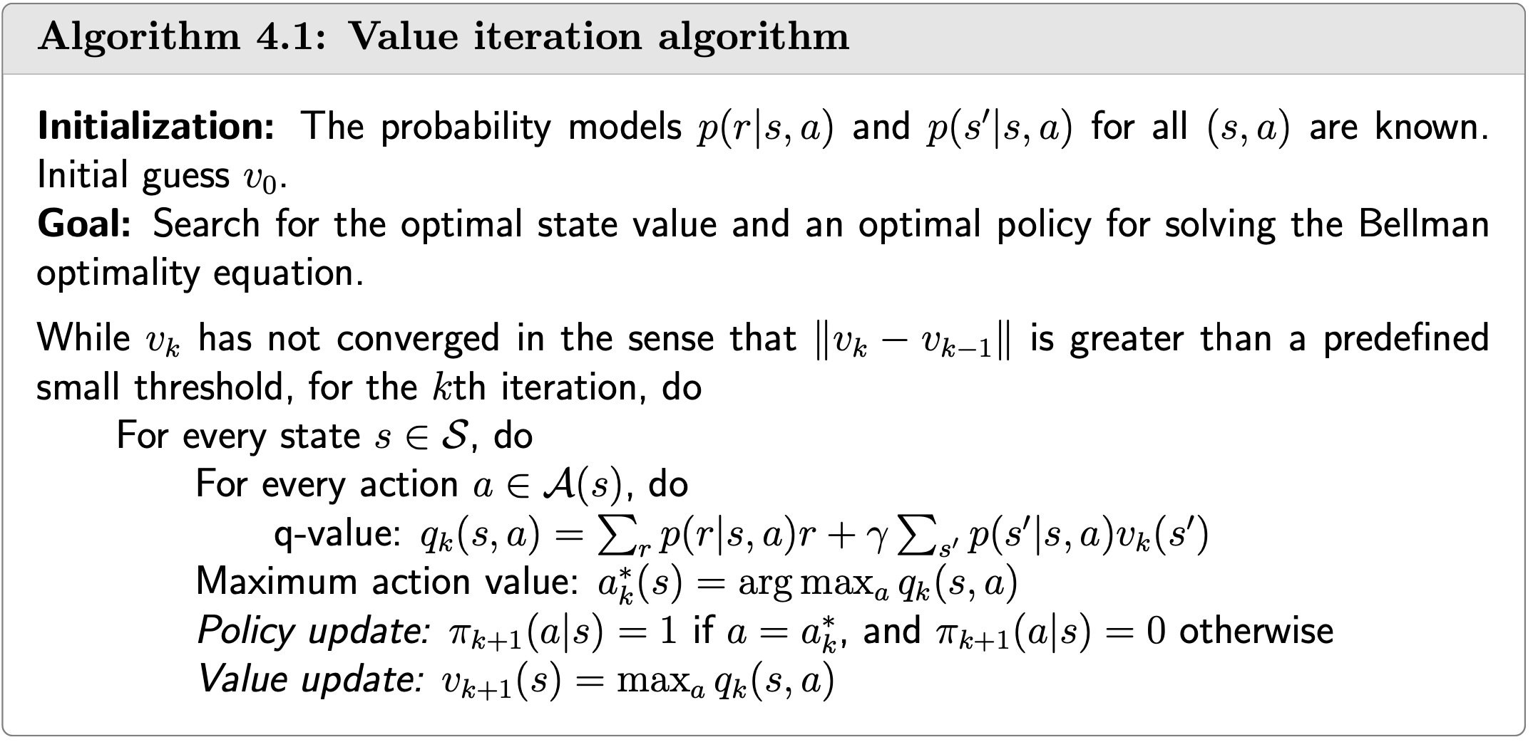
Recall from my earlier post, the elementwise form of \(\eqref{eq_policy_update}\) is \[ \pi_{k+1}(s)=\arg \max _\pi \sum_a \pi(a \mid s) \underbrace{\left(\sum_r p(r \mid s, a) r+\gamma \sum_{s^{\prime}} p\left(s^{\prime} \mid s, a\right) v_k\left(s^{\prime}\right)\right)}_{q_k(s, a)}, \quad s \in \mathcal{S} \]
The optimal policy solving the above optimization problem is \[ \pi_{k+1}(a \mid s)=\left\{\begin{array}{cc} 1 & a=a_k^*(s) \\ 0 & a \neq a_k^*(s) \end{array}\right. \] where \[ a_k^*(s)=\arg \max _a q_k(a, s) . \]
\(\pi_{k+1}\) is called a greedy policy, since it simply selects the greatest q-value.
Step 2
Step 2: Value update
The elementwise form of \(\eqref{eq_value_update}\) is \[ v_{k+1}(s)=\sum_a \pi_{k+1}(a \mid s) \underbrace{\left(\sum_r p(r \mid s, a) r+\gamma \sum_{s^{\prime}} p\left(s^{\prime} \mid s, a\right) v_k\left(s^{\prime}\right)\right)}_{q_k(s, a)}, \quad s \in \mathcal{S} \]
Since \(\pi_{k+1}\) is greedy, the above equation is simply \[ v_{k+1}(s)=\max _a q_k(a, s) \]
Algorithm
Procedure summary:
\(v_k(s) \rightarrow q_k(s, a) \rightarrow\) greedy policy \(\pi_{k+1}(a \mid s) \rightarrow\) new value \(v_{k+1}=\max _a q_k(s, a)\)
Now, since we get the optimal state-values, our optimal policy is clear-just selct the next state with the maximal state-value.
Example
We next present an example to illustrate the step-by-step implementation of the value iteration algorithm.
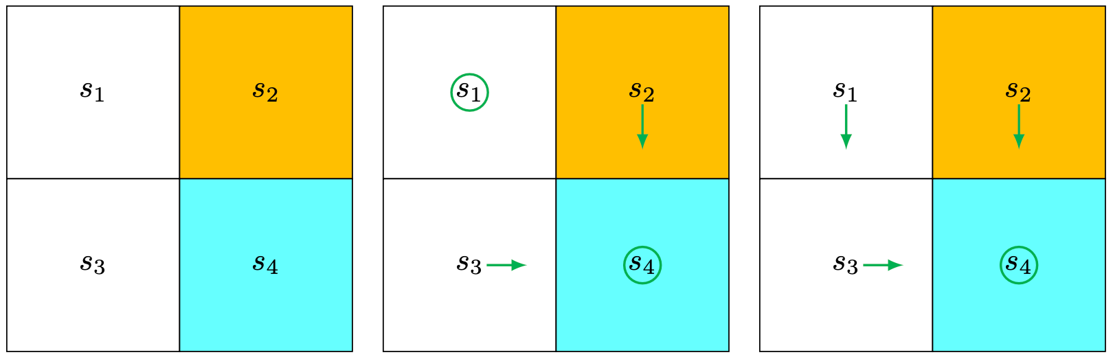 The target area is \(s_4\). The reward settings are \(r_{\text {boundary }}=r_{\text {forbidden }}=-1\) and \(r_{\text {target }}=1\). The discount rate is \(\gamma=0.9\).
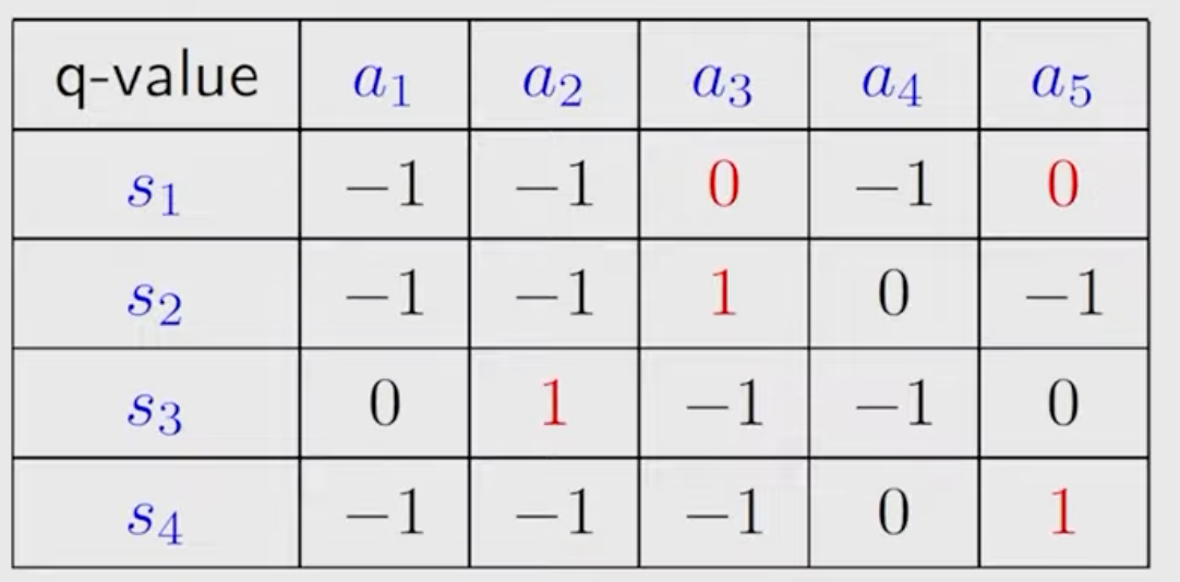
The q-table is:
%20for%20the%20example%20as%20shown%20in%20Figure%204_2.png)
k=0
\(k=0\) : let \(v_0\left(s_1\right)=v_0\left(s_2\right)=v_0\left(s_3\right)=v_0\left(s_4\right)=0\) 
Step 1: Policy update: \[ \pi_1\left(a_5 \mid s_1\right)=1, \pi_1\left(a_3 \mid s_2\right)=1, \pi_1\left(a_2 \mid s_3\right)=1, \pi_1\left(a_5 \mid s_4\right)=1 . \nonumber \]
This policy is visualized in Figure (b).
Step 2: Value update: \[ v_1\left(s_1\right)=0, v_1\left(s_2\right)=1, v_1\left(s_3\right)=1, v_1\left(s_4\right)=1 . \nonumber \]
k=1
\(k=1\) : since \[ v_1\left(s_1\right)=0, v_1\left(s_2\right)=1, v_1\left(s_3\right)=1, v_1\left(s_4\right)=1, \] we have
Step 1: Policy update:
\[ \pi_2\left(a_3 \mid s_1\right)=1, \pi_2\left(a_3 \mid s_2\right)=1, \pi_2\left(a_2 \mid s_3\right)=1, \pi_2\left(a_5 \mid s_4\right)=1 . \nonumber \]
Step 2: Value update:
\[ v_2\left(s_1\right)=\gamma 1, v_2\left(s_2\right)=1+\gamma 1, v_2\left(s_3\right)=1+\gamma 1, v_2\left(s_4\right)=1+\gamma 1 . \nonumber \]
This policy is visualized in Figure (c).
The policy is already optimal.
k=2,3,…
\(k=2,3, \ldots\) Stop when \(\left\|v_k-v_{k+1}\right\|\) is smaller than a predefined
Policy iteration
Policy iteration is an iterative algorithm. Each iteration has two steps.
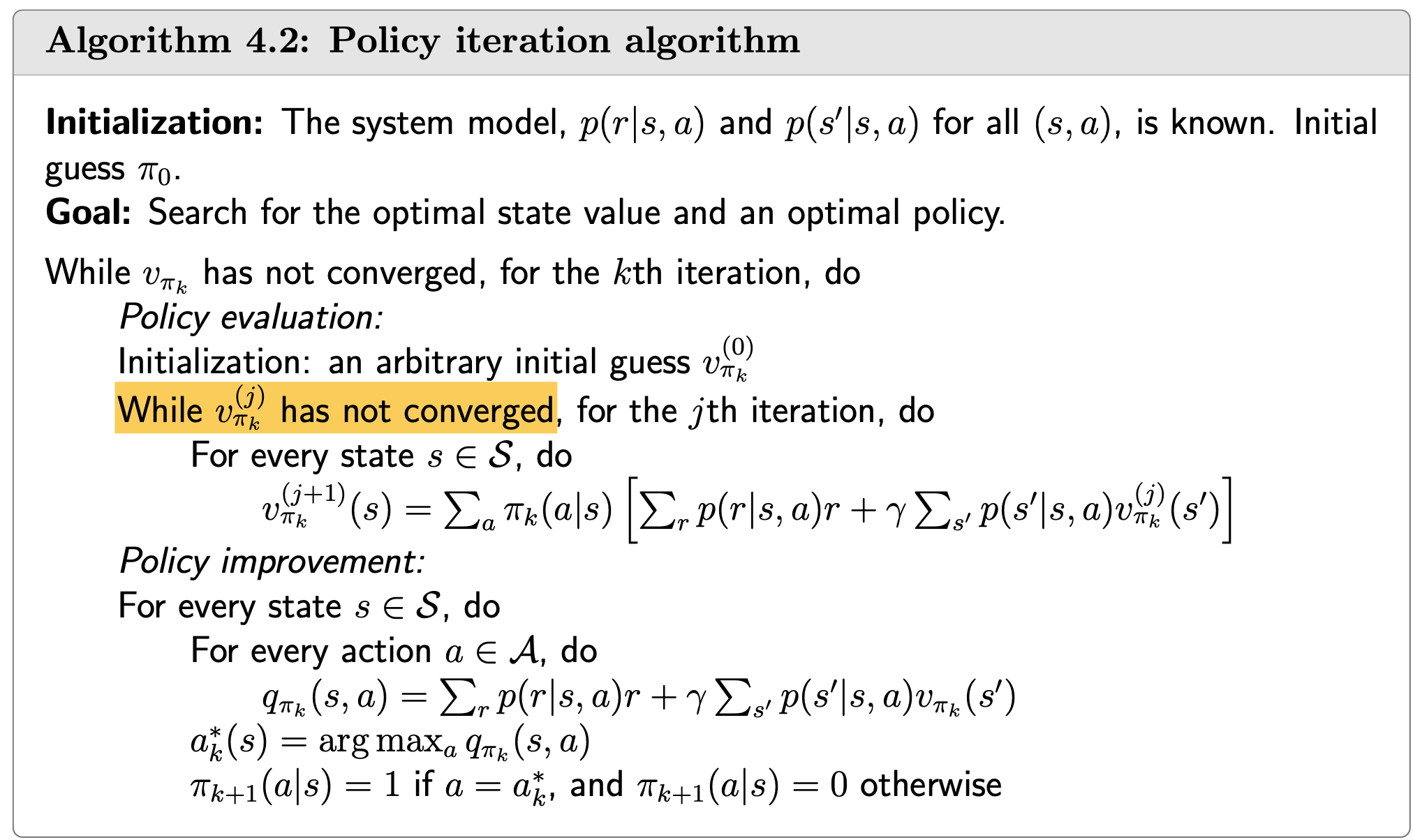
Given a random initial policy \(\pi_0\), in each olicy iteration we do
policy evaluation (PE): \[ \begin{equation} \label{eq_policy_evaluation} v_{\pi_k}=r_{\pi_k}+\gamma P_{\pi_k} v_{\pi_k} \end{equation} \] Note: \(v_{\pi_k}\) is a state value function. So we need to get the state values for all states, not for one specific state, in PE.
policy improvement (PI): \[ \pi_{k+1}=\arg \max _\pi\left(r_\pi+\gamma P_\pi v_{\pi_k}\right) \] The maximization is componentwise.
The policy iteration algorithm leads to a sequence \[ \pi_0 \stackrel{P E}{\longrightarrow} v_{\pi_0} \stackrel{P I}{\longrightarrow} \pi_1 \stackrel{P E}{\longrightarrow} v_{\pi_1} \stackrel{P I}{\longrightarrow} \pi_2 \stackrel{P E}{\longrightarrow} v_{\pi_2} \stackrel{P I}{\longrightarrow} \ldots \nonumber \]
Q1: In the policy evaluation step, how to calculate \(v_{\pi_k}\)?
\(\eqref{eq_policy_evaluation}\) is a Bellman equation. We’ve learned there’re two ways to solve it.
Closed-form solution: \[ v_{\pi_k}=\left(I-\gamma P_{\pi_k}\right)^{-1} r_{\pi_k} . \]
Iterative solution: \[ \begin{equation} \label{eq_iterative_solution} v_{\pi_k}^{(j+1)}=r_{\pi_k}+\gamma P_{\pi_k} v_{\pi_k}^{(j)}, \quad j=0,1,2, \ldots \end{equation} \]
where \(v_{\pi_k}^{(j)}\) denotes the \(j\) th estimate of \(v_{\pi_k}\). Starting from any initial guess \(v_{\pi_k}^{(0)}\), it is ensured that \(v_{\pi_k}^{(j)} \rightarrow v_{\pi_k}\) as \(j \rightarrow \infty\) (–>See the proof).
Interestingly, policy iteration is an iterative algorithm with another iterative algorithm \(\eqref{eq_iterative_solution}\) embedded in the policy evaluation step.
In theory, this embedded iterative algorithm requires an infinite number of steps (that is, \(j \rightarrow \infty\) ) to converge to the true state value \(v_{\pi_k}\). This is, however, impossible to realize.
In practice, the iterative process terminates when a certain criterion is satisfied.
Q2: In the policy improvement step, why is \(\pi_{k+1}\) better than \(\pi_k\) ?
Lemma (Policy improvement). If \(\pi_{k+1}=\arg \max _\pi\left(r_\pi+\gamma P_\pi v_{\pi_k}\right)\), then \(v_{\pi_{k+1}} \geq v_{\pi_k}\), which means \(v_{\pi_{k+1}}(s) \geq v_{\pi_k}(s)\) for all \(s\), i.e., \(\pi_{k+1}\) is better than \(\pi_k]\).
Proof: Since \(v_{\pi_{k+1}}\) and \(v_{\pi_k}\) are state values, they satisfy the Bellman equations: \[ \begin{aligned} v_{\pi_{k+1}} & =r_{\pi_{k+1}}+\gamma P_{\pi_{k+1}} v_{\pi_{k+1}}, \\ v_{\pi_k} & =r_{\pi_k}+\gamma P_{\pi_k} v_{\pi_k} . \end{aligned} \nonumber \]
Since \(\pi_{k+1}=\arg \max _\pi\left(r_\pi+\gamma P_\pi v_{\pi_k}\right)\), we know that \[ r_{\pi_{k+1}}+\gamma P_{\pi_{k+1}} v_{\pi_k} \geq r_{\pi_k}+\gamma P_{\pi_k} v_{\pi_k} \nonumber \] It then follows that \[ \begin{aligned} v_{\pi_k}-v_{\pi_{k+1}} & =\left(r_{\pi_k}+\gamma P_{\pi_k} v_{\pi_k}\right)-\left(r_{\pi_{k+1}}+\gamma P_{\pi_{k+1}} v_{\pi_{k+1}}\right) \\ & \leq\left(r_{\pi_{k+1}}+\gamma P_{\pi_{k+1}} v_{\pi_k}\right)-\left(r_{\pi_{k+1}}+\gamma P_{\pi_{k+1}} v_{\pi_{k+1}}\right) \\ & \leq \gamma P_{\pi_{k+1}}\left(v_{\pi_k}-v_{\pi_{k+1}}\right) . \end{aligned} \]
Therefore, \[ \begin{aligned} v_{\pi_k}-v_{\pi_{k+1}} \leq \gamma^2 P_{\pi_{k+1}}^2\left(v_{\pi_k}-v_{\pi_{k+1}}\right) \leq \ldots & \leq \gamma^n P_{\pi_{k+1}}^n\left(v_{\pi_k}-v_{\pi_{k+1}}\right) \\ & \leq \lim _{n \rightarrow \infty} \gamma^n P_{\pi_{k+1}}^n\left(v_{\pi_k}-v_{\pi_{k+1}}\right)=0 . \end{aligned} \]
The limit is due to the facts that \(\gamma^n \rightarrow 0\) as \(n \rightarrow \infty\) and \(P_{\pi_{k+1}}^n\) is a nonnegative stochastic matrix for any \(n\). Here, a stochastic matrix refers to a nonnegative matrix whose row sums are equal to one for all rows.
Q3: Why can the policy iteration algorithm eventually find an optimal policy?
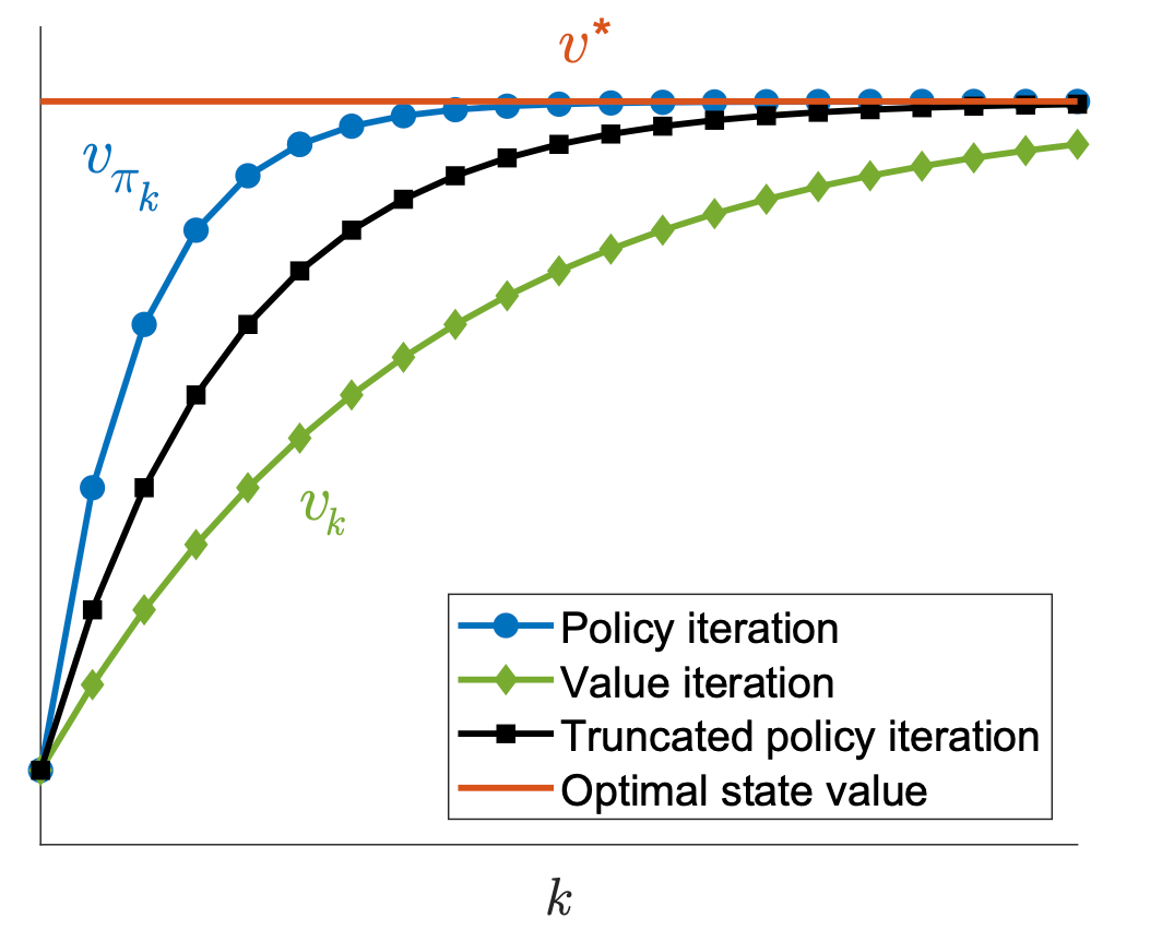
The policy iteration algorithm generates two sequences. The first is a sequence of policies: \(\left\{\pi_0, \pi_1, \ldots, \pi_k, \ldots\right\}\). The second is a sequence of state values: \(\left\{v_{\pi_0}, v_{\pi_1}, \ldots, v_{\pi_k}, \ldots\right\}\). Suppose that \(v^*\) is the optimal state value. Then, \(v_{\pi_k} \leq v^*\) for all \(k\).
Since the policies are continuously improved according to the previous Lemma, we know that \[ v_{\pi_0} \leq v_{\pi_1} \leq v_{\pi_2} \leq \cdots \leq v_{\pi_k} \leq \cdots \leq v^* \nonumber \]
Since \(v_{\pi_k}\) is nondecreasing and always bounded from above by \(v^*\), it follows from the monotone convergence theorem that \(v_{\pi_k}\) converges to a constant value, denoted as \(v_{\infty}\), when \(k \rightarrow \infty\).
Now we prove that \(v_{\infty}=v^*\).
Theorem (Convergence of policy iteration). The state value sequence \(\left\{v_{\pi_k}\right\}_{k=0}^{\infty}\) generated by the policy iteration algorithm converges to the optimal state value \(v^*\). As a result, the policy sequence \(\left\{\pi_k\right\}_{k=0}^{\infty}\) converges to an optimal policy.
Proof:
The idea of the proof is to show that the policy iteration algorithm converges faster than the value iteration algorithm.
In particular, to prove the convergence of \(\left\{v_{\pi_k}\right\}_{k=0}^{\infty}\), we introduce another sequence \(\left\{v_k\right\}_{k=0}^{\infty}\) generated by \[ v_{k+1}=f\left(v_k\right)=\max _\pi\left(r_\pi+\gamma P_\pi v_k\right) \]
This iterative algorithm is exactly the value iteration algorithm. We already know that \(v_k\) converges to \(v^*\) when given any initial value \(v_0\).
For \(k=0\), we can always find a \(v_0\) such that \(v_{\pi_0} \geq v_0\) for any \(\pi_0\).
We next show that \(v_k \leq v_{\pi_k} \leq v^*\) for all \(k\) by induction.
For \(k \geq 0\), suppose that \(v_{\pi_k} \geq v_k\).
For \(k+1\), we have \[ \begin{aligned} v_{\pi_{k+1}}-v_{k+1} & =\left(r_{\pi_{k+1}}+\gamma P_{\pi_{k+1}} v_{\pi_{k+1}}\right)-\max _\pi\left(r_\pi+\gamma P_\pi v_k\right) \\ & \geq\left(r_{\pi_{k+1}}+\gamma P_{\pi_{k+1}} v_{\pi_k}\right)-\max _\pi\left(r_\pi+\gamma P_\pi v_k\right) \end{aligned} \] (because \(v_{\pi_{k+1}} \geq v_{\pi_k}\) by Lemma 4.1 and \(P_{\pi_{k+1}} \geq 0\) ) \[ =\left(r_{\pi_{k+1}}+\gamma P_{\pi_{k+1}} v_{\pi_k}\right)-\left(r_{\pi_k^{\prime}}+\gamma P_{\pi_k^{\prime}} v_k\right) \nonumber \] (suppose \(\left.\pi_k^{\prime}=\arg \max _\pi\left(r_\pi+\gamma P_\pi v_k\right)\right)\) \[ \geq\left(r_{\pi_k^{\prime}}+\gamma P_{\pi_k^{\prime}} v_{\pi_k}\right)-\left(r_{\pi_k^{\prime}}+\gamma P_{\pi_k^{\prime}} v_k\right) \nonumber \] (because \(\pi_{k+1}=\arg \max _\pi\left(r_\pi+\gamma P_\pi v_{\pi_k}\right)\) ) \[ =\gamma P_{\pi_k^{\prime}}\left(v_{\pi_k}-v_k\right) \text {. } \nonumber \]
Since \(v_{\pi_k}-v_k \geq 0\) and \(P_{\pi_k^{\prime}}\) is nonnegative, we have \(P_{\pi_k^{\prime}}\left(v_{\pi_k}-v_k\right) \geq 0\) and hence \(v_{\pi_{k+1}}-v_{k+1} \geq 0\)
Therefore, we can show by induction that \(v_k \leq v_{\pi_k} \leq v^*\) for any \(k \geq 0\). Since \(v_k\) converges to \(v^*, v_{\pi_k}\) also converges to \(v^*\).
Elementwise form and implementation
Step 1
Step 1: Policy evaluation
Recalling the solution to do policy evaluation with matrix-vector form: \(\eqref{eq_iterative_solution}\).
The elementwise form is: \[ v_{\pi_k}^{(j+1)}(s)=\sum_a \pi_k(a \mid s)\left(\sum_r p(r \mid s, a) r+\gamma \sum_{s^{\prime}} p\left(s^{\prime} \mid s, a\right) v_{\pi_k}^{(j)}\left(s^{\prime}\right)\right), \quad s \in \mathcal{S}, \nonumber \]
Stop when \(j \rightarrow \infty\) or \(j\) is sufficiently large or \(\left\|v_{\pi_k}^{(j+1)}-v_{\pi_k}^{(j)}\right\|\) is sufficiently small.
Step 2
Step 2: Policy improvement Recalling the solution to do policy improvement with matrix-vector form: \(\pi_{k+1}=\arg \max _\pi\left(r_\pi+\gamma P_\pi v_{\pi_k}\right)\)
The elementwise form is: \[ \pi_{k+1}(s)=\arg \max _\pi \sum_a \pi(a \mid s) \underbrace{\left(\sum_r p(r \mid s, a) r+\gamma \sum_{s^{\prime}} p\left(s^{\prime} \mid s, a\right) v_{\pi_k}\left(s^{\prime}\right)\right)}_{q_{\pi_k}(s, a)}, \quad s \in \mathcal{S} . \nonumber \]
Here, \(q_{\pi_k}(s, a)\) is the action value under policy \(\pi_k\). Let \[ a_k^*(s)=\arg \max _a q_{\pi_k}(a, s) \nonumber \]
Then, the greedy policy is \[ \pi_{k+1}(a \mid s)= \begin{cases}1 & a=a_k^*(s), \\ 0 & a \neq a_k^*(s) .\end{cases} \nonumber \]
Algorithm
Example
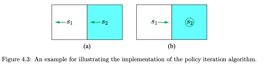
- The reward setting is \(r_{\text {boundary }}=-1\) and \(r_{\text {target }}=1\). The discount ate is \(\gamma=0.9\).
- Actions: \(a_{\ell}, a_0, a_r\) represent go left, stay unchanged, and go right.
- Aim: use policy iteration to find out the optimal policy.
k=0
Iteration \(k=0\) :
Step 1: policy evaluation \(\pi_0\) is selected as the policy in Figure (a). The Bellman equation is \[ \begin{aligned} & v_{\pi_0}\left(s_1\right)=-1+\gamma v_{\pi_0}\left(s_1\right), \\ & v_{\pi_0}\left(s_2\right)=0+\gamma v_{\pi_0}\left(s_1\right) . \end{aligned} \]
Since the quation is simple, it can be manually solved that \[ v_{\pi_0}\left(s_1\right)=-10, \quad v_{\pi_0}\left(s_2\right)=-9 . \]
In practice, the equation can be solved by the iterative algorithm in \(\eqref{eq_iterative_solution}\). For example, select the initial state values as \(v_{\pi_0}^{(0)}\left(s_1\right)=v_{\pi_0}^{(0)}\left(s_2\right)=0\). It follows from \(\eqref{eq_policy_evaluation}\) that: $$ \[\begin{aligned} & \left\{\begin{array}{l} v_{\pi_0}^{(1)}\left(s_1\right)=-1+\gamma v_{\pi_0}^{(0)}\left(s_1\right)=-1, \\ v_{\pi_0}^{(1)}\left(s_2\right)=0+\gamma v_{\pi_0}^{(0)}\left(s_1\right)=0, \end{array}\right. \\ & \left\{\begin{array}{l} v_{\pi_0}^{(2)}\left(s_1\right)=-1+\gamma v_{\pi_0}^{(1)}\left(s_1\right)=-1.9, \\ v_{\pi_0}^{(2)}\left(s_2\right)=0+\gamma v_{\pi_0}^{(1)}\left(s_1\right)=-0.9, \end{array}\right. \\ & \left\{\begin{array}{l} v_{\pi_0}^{(3)}\left(s_1\right)=-1+\gamma v_{\pi_0}^{(2)}\left(s_1\right)=-2.71, \\ v_{\pi_0}^{(3)}\left(s_2\right)=0+\gamma v_{\pi_0}^{(2)}\left(s_1\right)=-1.71, \end{array}\right. \\ &\cdots \end{aligned}\]$$
With more iterations, we can see the trend: \(v_{\pi_0}^{(j)}\left(s_1\right) \rightarrow v_{\pi_0}\left(s_1\right)=-10\) and \(v_{\pi_0}^{(j)}\left(s_2\right) \rightarrow\) \(v_{\pi_0}\left(s_2\right)=-9\) as \(j\) increases.
Step 2: policy improvement
The expression of \(q_{\pi_k}(s, a)\) :
| \(q_{\pi_k}(s, a)\) | \(a_{\ell}\) | \(a_0\) | \(a_r\) |
|---|---|---|---|
| \(s_1\) | \(-1+\gamma v_{\pi_k}\left(s_1\right)\) | \(0+\gamma v_{\pi_k}\left(s_1\right)\) | \(1+\gamma v_{\pi_k}\left(s_2\right)\) |
| \(s_2\) | \(0+\gamma v_{\pi_k}\left(s_1\right)\) | \(1+\gamma v_{\pi_k}\left(s_2\right)\) | \(-1+\gamma v_{\pi_k}\left(s_2\right)\) |
Substituting \(v_{\pi_0}\left(s_1\right)=-10, v_{\pi_0}\left(s_2\right)=-9\) and \(\gamma=0.9\) obtained in the previous policy evaluation
step into the above table yields:
| \(q_{\pi_0}(s, a)\) | \(a_{\ell}\) | \(a_0\) | \(a_r\) |
|---|---|---|---|
| \(s_1\) | -10 | -9 | -7.1 |
| \(s_2\) | -9 | -7.1 | -9.1 |
By seeking the greatest value of \(q_{\pi_0}\), the improved policy is: \[ \pi_1\left(a_r \mid s_1\right)=1, \quad \pi_1\left(a_0 \mid s_2\right)=1 \nonumber \]
This policy is optimal after one iteration! In your programming, should continue until the stopping criterion is satisfied.
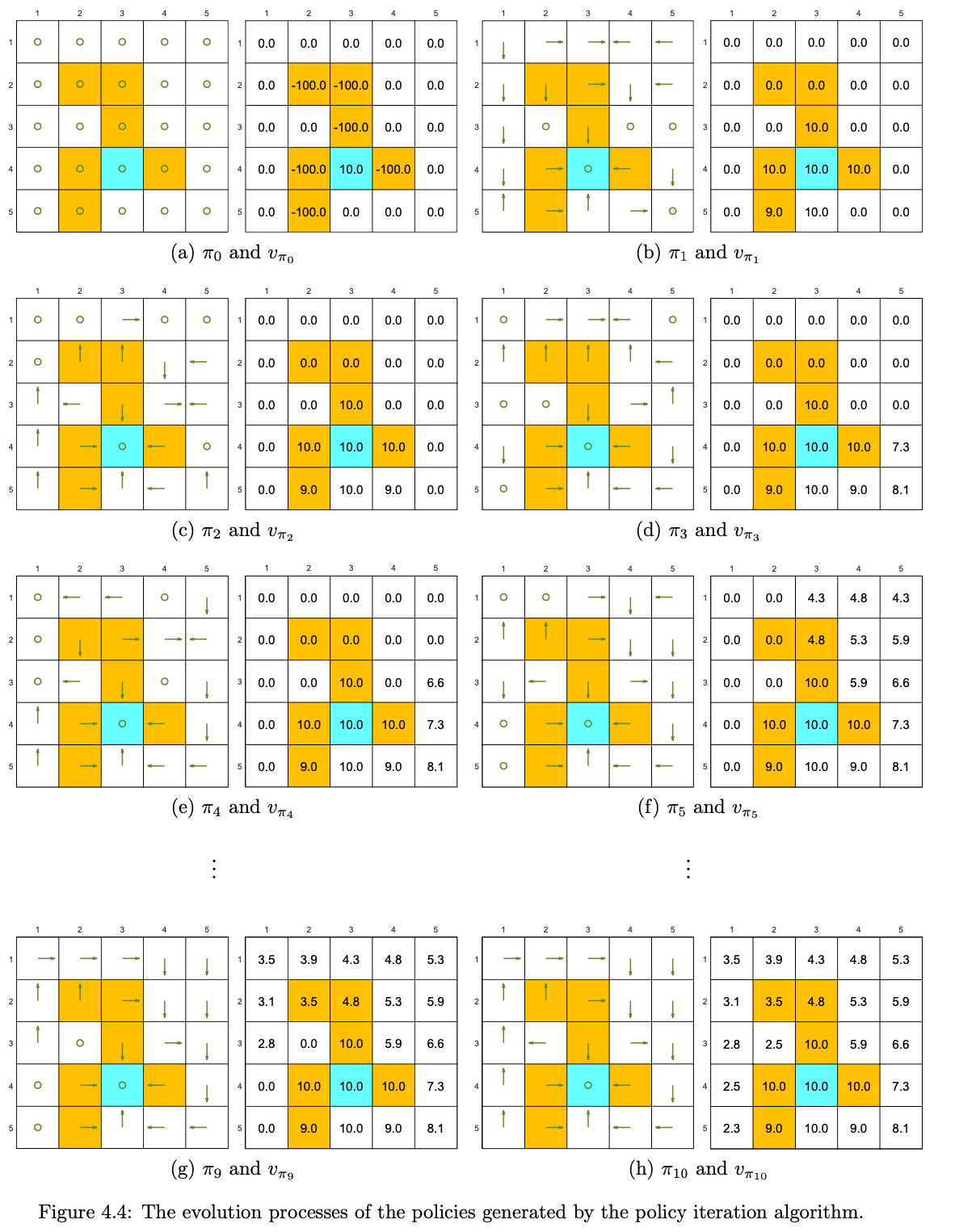
A more complicated example
Setting \(r_{\text {boundary }}=-1, r_{\text {forbidden }}=-10\), and \(r_{\text {target }}=\) 1. The discount rate is \(\gamma=0.9\). The policy iteration algorithm can converge to the optimal policy (Figure 4.4(h)) when starting from a random initial policy (Figure 4.4(a)).
Truncated policy iteration
The above steps of the two algorithms can be illustrated as
Policy iteration: \(\pi_0 \xrightarrow{P E} v_{\pi_0} \xrightarrow{P I} \pi_1 \xrightarrow{P E} v_{\pi_1} \xrightarrow{P I} \pi_2 \xrightarrow{P E} v_{\pi_2} \xrightarrow{P I} \ldots\).
Value iteration: \(\quad v_0 \xrightarrow{P U} \pi_1^{\prime} \xrightarrow{V U} v_1 \xrightarrow{P U} \pi_2^{\prime} \xrightarrow{V U} v_2 \xrightarrow{P U} \ldots\)
It can be seen that the procedures of the two algorithms are very similar. We examine their value steps more closely to see the difference between the two algorithms. In particular, let both algorithms start from the same initial condition: \(v_0=v_{\pi_0}\).
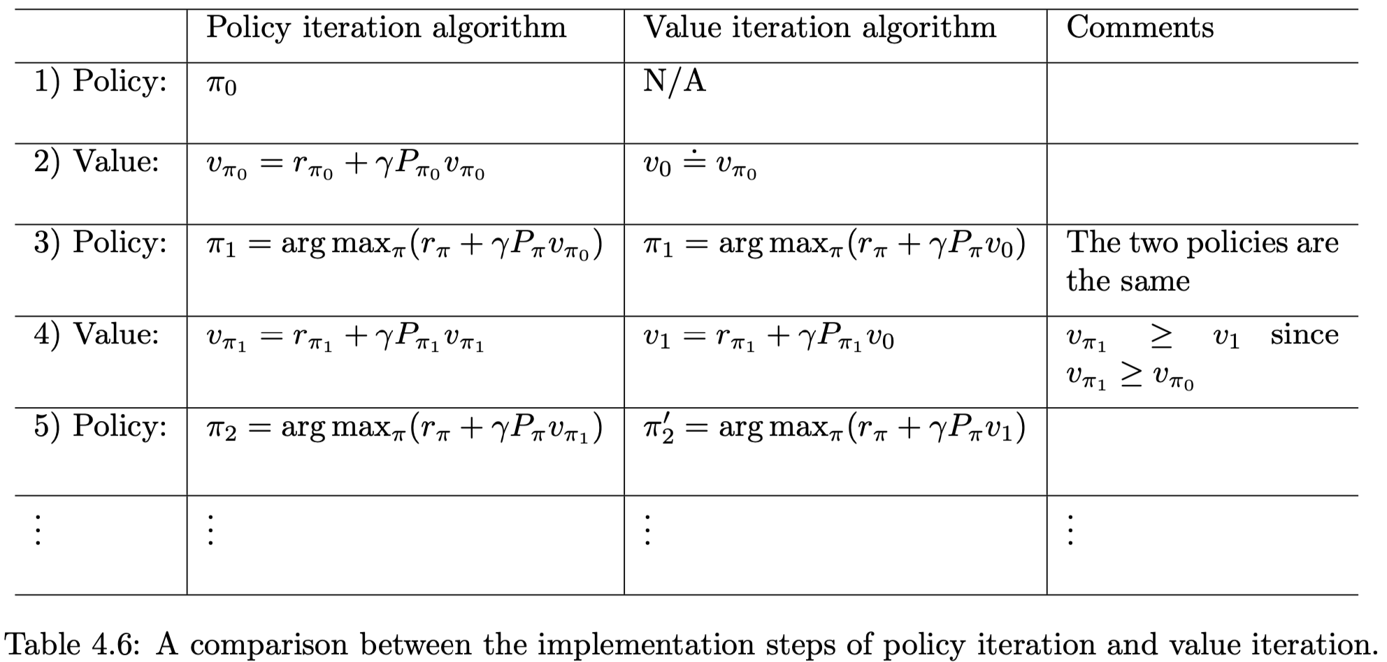
The procedures of the two algorithms are listed in Table 4.6.
- In the first three steps, the two algorithms generate the same results since \(v_0=v_{\pi_0}\). They become different in the fourth step.
- During the fourth step, the value iteration algorithm executes \(v_1=r_{\pi_1}+\gamma P_{\pi_1} v_0\), which is a one-step calculation, whereas the policy iteration algorithm solves \(v_{\pi_1}=r_{\pi_1}+\gamma P_{\pi_1} v_{\pi_1}\), which requires an infinite number of iterations.
If we explicitly write out the iterative process for solving \(v_{\pi_1}=r_{\pi_1}+\gamma P_{\pi_1} v_{\pi_1}\) in the fourth step, everything becomes clear. By letting \(v_{\pi_1}^{(0)}=v_0\), we have
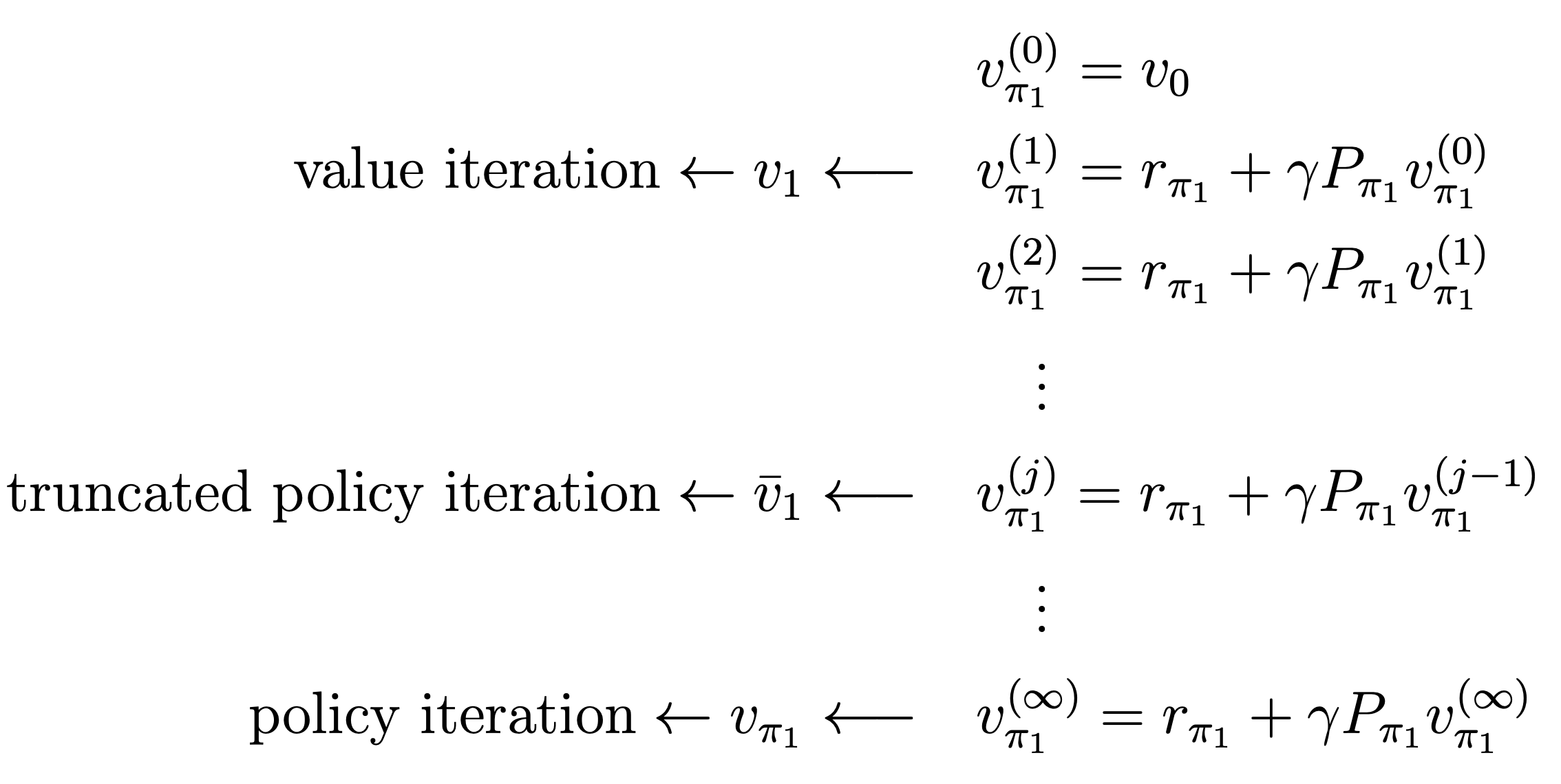
The following observations can be obtained from the above process.
- If the iteration is run only once, then \(v_{\pi_1}^{(1)}\) is actually \(v_1\), as calculated in the value iteration algorithm.
- eration is run an infinite number of times, then \(v_{\pi_1}^{(\infty)}\) is actually \(v_{\pi_1}\), as calculated in the policy iteration algorithm.
- If the iteration is run a finite number of times (denoted as \(j_{\text {truncate }}\) ), then such an algorithm is called truncated policy iteration. It is called truncated because the remaining iterations from \(j_{\text {truncate }}\) to \(\infty\) are truncated.
As a result, the value iteration and policy iteration algorithms can be viewed as two extreme cases of the truncated policy iteration algorithm: value iteration terminates at \(j_{\text {truncate }}=1\), and policy iteration terminates at \(j_{\text {truncate }}=\infty\).
It should be noted that, although the above comparison is illustrative, it is based on the condition that \(v_{\pi_1}^{(0)}=v_0=v_{\pi_0}\). The two algorithms cannot be directly compared without this condition.
Truncated policy iteration algorithm
In a nutshell, the truncated policy iteration algorithm is the same as the policy iteration algorithm except that it merely runs a finite number of iterations in the policy evaluation step.
Lemma: Value Improvement
Consider the iterative algorithm for solving the policy evaluation step: \[ v_{\pi_k}^{(j+1)}=r_{\pi_k}+\gamma P_{\pi_k} v_{\pi_k}^{(j)}, \quad j=0,1,2, \ldots \]
If the initial guess is selected as \(v_{\pi_k}^{(0)}=v_{\pi_{k-1}}\), it holds that \[ v_{\pi_k}^{(j+1)} \geq v_{\pi_k}^{(j)} \] for every \(j=0,1,2, \ldots\).
Proof: First, since \(v_{\pi_k}^{(j)}=r_{\pi_k}+\gamma P_{\pi_k} v_{\pi_k}^{(j-1)}\) and \(v_{\pi_k}^{(j+1)}=r_{\pi_k}+\gamma P_{\pi_k} v_{\pi_k}^{(j)}\), we have \[ v_{\pi_k}^{(j+1)}-v_{\pi_k}^{(j)}=\gamma P_{\pi_k}\left(v_{\pi_k}^{(j)}-v_{\pi_k}^{(j-1)}\right)=\cdots=\gamma^j P_{\pi_k}^j\left(v_{\pi_k}^{(1)}-v_{\pi_k}^{(0)}\right) \]
Second, since \(v_{\pi_k}^{(0)}=v_{\pi_{k-1}}\), we have \[ v_{\pi_k}^{(1)}=r_{\pi_k}+\gamma P_{\pi_k} v_{\pi_k}^{(0)}=r_{\pi_k}+\gamma P_{\pi_k} v_{\pi_{k-1}} \geq r_{\pi_{k-1}}+\gamma P_{\pi_{k-1}} v_{\pi_{k-1}}=v_{\pi_{k-1}}=v_{\pi_k}^{(0)}, \] where the inequality is due to \(\pi_k=\arg \max _\pi\left(r_\pi+\gamma P_\pi v_{\pi_{k-1}}\right)\). Substituting \(v_{\pi_k}^{(1)} \geq v_{\pi_k}^{(0)}\) into (4.5) yields \(v_{\pi_k}^{(j+1)} \geq v_{\pi_k}^{(j)}\).
TODO
There’s no proof of truncated policy iteration can produce the optimal policy….
Relationships between the three algorithms