Bellman Optimality Equation

Posted on 2024-01-07 Edited on 2024-05-09 In Computer Science Views:

Optimal Policy

The state value could be used to evaluate if a policy is good or not: if \[ v_{\pi_1}(s) \geq v_{\pi_2}(s) \quad \text { for all } s \in \mathcal{S} \] then \(\pi_1\) is "better" than \(\pi_2\).

A policy \(\pi^*\) is optimal if \(v_{\pi^*}(s) \geq v_\pi(s)\) for all \(s\) and for any other policy \(\pi\).

The definition leads to many questions:

Does the optimal policy exist?
Is the optimal policy unique?
Is the optimal policy stochastic or deterministic?
How to obtain the optimal policy?

To answer these questions, we study the Bellman optimality equation.

BOE (elementwise form)

The tool for analyzing optimal policies and optimal state values is the Bellman optimality equation (BOE). By solving this equation, we can obtain optimal policies and optimal state values.

For every \(s \in \mathcal{S}\), the elementwise expression of the BOE is \[ \begin{aligned} v(s) & =\max _{\pi(s) \in \Pi(s)} \sum_{a \in \mathcal{A}} \pi(a \mid s)\left(\sum_{r \in \mathcal{R}} p(r \mid s, a) r+\gamma \sum_{s^{\prime} \in \mathcal{S}} p\left(s^{\prime} \mid s, a\right) v\left(s^{\prime}\right)\right) \\ & =\max _{\pi(s) \in \Pi(s)} \sum_{a \in \mathcal{A}} \pi(a \mid s) q(s, a), \end{aligned} \] where \(v(s), v\left(s^{\prime}\right)\) are unknown variables to be solved and \[ q(s, a) \doteq \sum_{r \in \mathcal{R}} p(r \mid s, a) r+\gamma \sum_{s^{\prime} \in \mathcal{S}} p\left(s^{\prime} \mid s, a\right) v\left(s^{\prime}\right) \]

Here, \(\pi(s)\) denotes a policy for state \(s\), and \(\Pi(s)\) is the set of all possible policies for \(s\).

Remarks:

\(p(r \mid s, a), p\left(s^{\prime} \mid s, a\right)\) are known.

\(v(s), v\left(s^{\prime}\right)\) are unknown and to be calculated.

Maximize on the right-hand side of BOE

Here we talk about how to solve BOE. In practice we need to deal with the matrix-vector form since that is what we're faced with. But since each row in the matrix is actually a vector of the elementwise form, we start with the element form.

In fact, we can turn the problem into "solve the optimal \(\pi\) on the right-hand side". Let's look at one example first:

Example 3.1. Consider two unknown variables \(x, y \in \mathbb{R}\) that satisfy \[ x=\max _{y \in \mathbb{R}}\left(2 x-1-y^2\right) . \]

The first step is to solve \(y\) on the right-hand side of the equation. Regardless of the value of \(x\), we always have \(\max _y\left(2 x-1-y^2\right)=2 x-1\), where the maximum is achieved when \(y=0\). The second step is to solve \(x\). When \(y=0\), the equation becomes \(x=2 x-1\), which leads to \(x=1\). Therefore, \(y=0\) and \(x=1\) are the solutions of the equation.

We now turn to the maximization problem on the right-hand side of the BOE. The (elementwise) BOE can be written as \[ v(s)=\max _{\pi(s) \in \Pi(s)} \sum_{a \in \mathcal{A}} \pi(a \mid s) q(s, a), \quad s \in \mathcal{S} . \]

Inspired by Example 3.1, we can first solve the optimal \(\pi\) on the right-hand side. How to do that? The following example demonstrates its basic idea.

Example 3.2. Given \(q_1, q_2, q_3 \in \mathbb{R}\), we would like to find the optimal values of \(c_1, c_2, c_3\) to maximize \[ \sum_{i=1}^3 c_i q_i=c_1 q_1+c_2 q_2+c_3 q_3, \] where \(c_1+c_2+c_3=1\) and \(c_1, c_2, c_3 \geq 0\). Without loss of generality, suppose that \(q_3 \geq q_1, q_2\). Then, the optimal solution is \(c_3^*=1\) and \(c_1^*=c_2^*=0\). This is because \[ q_3=\left(c_1+c_2+c_3\right) q_3=c_1 q_3+c_2 q_3+c_3 q_3 \geq c_1 q_1+c_2 q_2+c_3 q_3 \] for any \(c_1, c_2, c_3\).

Inspired by the above example, considering that \(\sum_a \pi(a \mid s)=1\), we have \[ \begin{equation} \label{eq_elementwise_form_right} v(s) = \max _\pi \sum_a \pi(a \mid s) q(s, a)=\max _{a \in \mathcal{A}(s)} q(s, a) \end{equation} \] where the optimality is achieved when \[ \pi(a \mid s)= \begin{cases}1 & a=a^* \\ 0 & a \neq a^*\end{cases} \] where \(a^*=\arg \max _a q(s, a)\).

Now that we know the solution of BOE is to maximize the right-hand side, and we know how to do it as well --- just select the action with the largest action value. But we don't know action value or state value at this time, so this method doesn't work.

In fact, the solution of BOE derives from the contraction mapping theorem (see later) on the matrix-vector form. That's an iterative method

So why we introduce \(\eqref{eq_elementwise_form_right}\) here? The reason at during every iteration, for every state \(s\), the action value will already have been known, so we can use \(\eqref{eq_elementwise_form_right}\) to get the maximized right-hand side, which is the maximized \(v(s)\)!

Matrix-vector form of the BOE

To leverage the contraction mapping theorem, we'll express the matrix-vector form as \(v = f(v)\).

Since the optimal value of \(\pi\) is determined by \(v\), the right-hand side of BOE (matrix-vector form) is a function of \(v\), denoted as \[ \begin{equation} \label{eq_right_hand_side} f(v) \triangleq \max _{\pi}\left(r_\pi+\gamma P_\pi v\right) . \end{equation} \]

where \(v \in \mathbb{R}^{|\mathcal{S}|}\) and \(\max _\pi\) is performed in an elementwise manner. The structures of \(r_\pi\) and \(P_\pi\) are the same as those in the matrix-vector form of the normal Bellman equation: \[ \left[r_\pi\right]_s \doteq \sum_{a \in \mathcal{A}} \pi(a \mid s) \sum_{r \in \mathcal{R}} p(r \mid s, a) r, \quad\left[P_\pi\right]_{s, s^{\prime}}=p\left(s^{\prime} \mid s\right) \doteq \sum_{a \in \mathcal{A}} \pi(a \mid s) p\left(s^{\prime} \mid s, a\right) . \]

Then, the BOE can be expressed in a concise form as \[ v=f(v) \]

Every row \([f(v)]_s\) is the elementwise form of \(s\).

Contraction mapping theorem

Now that the matrix-vector form is expressed as a nonlinear equation \(v = f(v)\), we next introduce the contraction mapping theorem to analyze it.

Concepts: Fixed point and Contraction mapping

Fixed point: \(x \in X\) is a fixed point of \(f: X \rightarrow X\) if \[ f(x)=x \] ***

Contraction mapping (or contractive function): \(f\) is a contraction mapping if \[ \left\|f\left(x_1\right)-f\left(x_2\right)\right\| \leq \gamma\left\|x_1-x_2\right\| \] where \(\gamma \in(0,1)\). - \(\gamma\) must be strictly less than 1 so that many limits such as \(\gamma^k \rightarrow 0\) as \(k \rightarrow 0\) hold. - Here \(\|\cdot\|\) can be any vector norm.

Example1

Givn euqation: \[ x=f(x)=0.5 x, x \in \mathbb{R} . \] It is easy to verify that \(x=0\) is a fixed point since \(0=0.5 \times 0\). Moreover, \(f(x)=0.5 x\) is a contraction mapping because \[ \left\|0.5 x_1-0.5 x_2\right\|=0.5\left\|x_1-x_2\right\| \leq \gamma\left\|x_1-x_2\right\| \] for any \(\gamma \in[0.5,1)\).

Example2

Given \(x=f(x)=A x\), where \(x \in \mathbb{R}^n, A \in \mathbb{R}^{n \times n}\) and \(\|A\| \leq \gamma<1\). It is easy to verify that \(x=0\) is a fixed point since \(0=A 0\). To see the contraction property, \[ \left\|A x_1-A x_2\right\|=\left\|A\left(x_1-x_2\right)\right\| \leq\|A\|\left\|x_1-x_2\right\| \leq \gamma\left\|x_1-x_2\right\| . \]

Therefore, \(f(x)=A x\) is a contraction mapping.

Theorem: Contraction Mapping Theorem

Theorem (Contraction Mapping Theorem): For any equation that has the form of \(x=f(x)\), if \(f\) is a contraction mapping, then

Existence: there exists a fixed point \(x^*\) satisfying \(f\left(x^*\right)=x^*\).
Uniqueness: The fixed point \(x^*\) is unique.
Algorithm: Consider a sequence \(\left\{x_k\right\}\) where \(x_{k+1}=f\left(x_k\right)\), then \(x_k \rightarrow x^*\) as \(k \rightarrow \infty\). Moreover, the convergence rate is exponentially fast.

-> See the proof

Contraction property of BOE

Theorem (Contraction Property):

\(f(v)\) in \(\eqref{eq_right_hand_side}\) is a contraction mapping satisfying \[ \left\|f\left(v_1\right)-f\left(v_2\right)\right\| \leq \gamma\left\|v_1-v_2\right\| \] where \(\gamma \in(0,1)\) is the discount rate, and \(\|\cdot\|_{\infty}\) is the maximum norm, which is the maximum absolute value of the elements of a vector.

-> See the proof

Solution of the BOE

Due to the contraction property of BOE, the matrix-vector form can be solved by computing following equation iteratively \[ \begin{equation} \label{eq_solution_for_elementwise_form} v_{k+1}=f\left(v_k\right)=\max _\pi\left(r_\pi+\gamma P_\pi v_k\right) . \end{equation} \]

At every iteration, for each state, what we face is actually the elementwise form:

\[ \begin{aligned} v_{k+1}(s) & =\max _\pi \sum_a \pi(a \mid s)\left(\sum_r p(r \mid s, a) r+\gamma \sum_{s^{\prime}} p\left(s^{\prime} \mid s, a\right) v_k\left(s^{\prime}\right)\right) \\ & =\max _\pi \sum_a \pi(a \mid s) q_k(s, a) \\ & =\max _a q_k(s, a) . \end{aligned} \]

As you can see, \(\eqref{eq_elementwise_form_right}\) is leveraged here. (But I don't know why can I do it. There's no proof about the contraction property of elementwise form, only one for the matrix-vector form)

Procedure summary (value iteration algorithm):

For every \(s\), estimate(randomly select) current state value as \(v_k(s)\)
For any \(a \in \mathcal{A}(s)\), calculate \[ q_k(s, a)=\sum_r p(r \mid s, a) r+\gamma \sum_{s^{\prime}} p\left(s^{\prime} \mid s, a\right) v_k\left(s^{\prime}\right) \]
Calculate the greedy policy \(\pi_{k+1}\) for every \(s\) as \[ \pi_{k+1}(a \mid s)=\left\{\begin{array}{cc} 1 & a=a_k^*(s) \\ 0 & a \neq a_k^*(s) \end{array}\right. \] where \(a_k^*(s)=\arg \max _a q_k(s, a)\).
Calculate \(v_{k+1}(s)=\max _a q_k(s, a)\)

Example

Example: Manually solve the BOE.

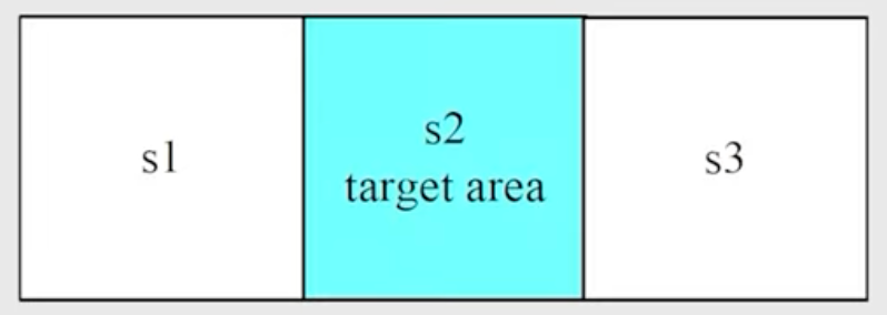
Actions: \(a_{\ell}, a_0, a_r\) represent go left, stay unchanged, and go right.
Reward: entering the target area: +1 ; try to go out of boundary -1.

The values of \(q(s, a)\):

q-value table	\(a_{\ell}\)	\(a_0\)	\(a_r\)
\(s_1\)	\(-1+\gamma v\left(s_1\right)\)	\(0+\gamma v\left(s_1\right)\)	\(1+\gamma v\left(s_2\right)\)
\(s_2\)	\(0+\gamma v\left(s_1\right)\)	\(1+\gamma v\left(s_2\right)\)	\(0+\gamma v\left(s_3\right)\)
\(s_3\)	\(1+\gamma v\left(s_2\right)\)	\(0+\gamma v\left(s_3\right)\)	\(-1+\gamma v\left(s_3\right)\)

Consider \(\gamma=0.9\).

Our objective is to find \(v^*\left(s_i\right)\) and \(\pi^*\):

\(k=0\):

v-value: select \(v_0\left(s_1\right)=v_0\left(s_2\right)=v_0\left(s_3\right)=0\)

q-value (using the previous table):

q-value table	\(a_{\ell}\)	\(a_0\)	\(a_r\)
\(s_1\)	-1	0	1
\(s_2\)	0	1	0
\(s_3\)	1	0	-1

Greedy policy (select the greatest q-value) \[ \pi\left(a_r \mid s_1\right)=1, \quad \pi\left(a_0 \mid s_2\right)=1, \quad \pi\left(a_{\ell} \mid s_3\right)=1 \] v-value: \(v_1(s)=\max _a q_0(s, a)\) \[ v_1\left(s_1\right)=v_1\left(s_2\right)=v_1\left(s_3\right)=1 \]

\(k=1\):

With \(v_1(s)\) calculated in the last step, q-value:

q-value table	\(a_{\ell}\)	\(a_0\)	\(a_r\)
\(s_1\)	-0.1	0.9	1.9
\(s_2\)	0.9	1.9	0.9
\(s_3\)	1.9	0.9	-0.1

Greedy policy (select the greatest q-value): \[ \pi\left(a_r \mid s_1\right)=1, \quad \pi\left(a_0 \mid s_2\right)=1, \quad \pi\left(a_{\ell} \mid s_3\right)=1 \]

The policy is the same as the previous one, which is already optimal. v-value: \(v_2(s)=\ldots\)

\(k=2,3, \ldots\), iterate until the produced q-value doesn't change too much.

BOE: Optimality

Suppose \(v^*\) is the solution to the Bellman optimality equation. It satisfies \[ v^*=\max _\pi\left(r_\pi+\gamma P_\pi v^*\right) \]

Suppose \[ \pi^*=\arg \max _\pi\left(r_\pi+\gamma P_\pi v^*\right) \]

Then \[ v^*=r_{\pi^*}+\gamma P_{\pi^*} v^* \]

Therefore, \(\pi^*\) is a policy and \(v^*=v_{\pi^*}\) is the corresponding state value.

Now we prove \(\pi^*\) is the optilmal policy:

Theorem (Policy Optimality):

Suppose that \(v^*\) is the unique solution to \(v=\max _\pi\left(r_\pi+\gamma P_\pi v\right)\), and \(v_\pi\) is the state value function satisfying \(v_\pi=r_\pi+\gamma P_\pi v_\pi\) for any given policy \(\pi\), then \[ v^* \geq v_\pi, \quad \forall \pi \] -> See the proof

What does \(\pi^\star\) look like?

For any \(s \in \mathcal{S}\), the deterministic greedy policy \[ \pi^*(a \mid s)= \begin{cases}1 & a=a^*(s) \\ 0 & a \neq a^*(s)\end{cases} \] is an optimal policy solving the BOE. Here, \[ a^*(s)=\arg \max _a q^*(a, s) \] where \(q^*(s, a):=\sum_r p(r \mid s, a) r+\gamma \sum_{s^{\prime}} p\left(s^{\prime} \mid s, a\right) v^*\left(s^{\prime}\right)\).

Proof: Due to \[ \pi^*(s)=\arg \max _{\pi \in \Pi} \sum_{a \in \mathcal{A}} \pi(a \mid s) \underbrace{\left(\sum_{r \in \mathcal{R}} p(r \mid s, a) r+\gamma \sum_{s^{\prime} \in \mathcal{S}} p\left(s^{\prime} \mid s, a\right) v^*\left(s^{\prime}\right)\right)}_{q^*(s, a)}, \quad s \in \mathcal{S} . \]

It is clear that \(\sum_{a \in \mathcal{A}} \pi(a \mid s) q^*(s, a)\) is maximized if \(\pi(s)\) selects the action with the greatest \(q^*(s, a)\).

Theorem: Optimal policy invariance

Theorem (Optimal policy invariance):

Consider a Markov decision process with \(v^* \in \mathbb{R}^{|\mathcal{S}|}\) as the optimal state value satisfying \(v^*=\max _{\pi \in \Pi}\left(r_\pi+\gamma P_\pi v^*\right)\). If every reward \(r \in \mathcal{R}\) is changed by an affine transformation to \(\alpha r+\beta\), where \(\alpha, \beta \in \mathbb{R}\) and \(\alpha>0\), then the corresponding optimal state value \(v^{\prime}\) is also an affine transformation of \(v^*\) : \[ v^{\prime}=\alpha v^*+\frac{\beta}{1-\gamma} \mathbf{1} \] where \(\gamma \in(0,1)\) is the discount rate and \(\mathbf{1}=[1, \ldots, 1]^T\).

Consequently, the optimal policy derived from \(v^{\prime}\) is invariant to the affine transformation of the reward values.

-> See the proof

Appendix

Proof of the contraction mapping theorem

Part 1

We prove that the consequence \(\left\{x_k\right\}_{k=1}^{\infty}\) with \(x_k=f\left(x_{k-1}\right)\) is convergent.

The proof relies on Cauchy sequences:

A sequence \(x_1, x_2, \cdots \in \mathbb{R}\) is called Cauchy if for any small \(\varepsilon>0\), there exists \(N\) such that \(\left\|x_m-x_n\right\|<\varepsilon\) for all \(m, n>N\).

It is guaranteed that a Cauchy sequence converges to a limit.

Note that we must have \(\left\|x_m-x_n\right\|<\varepsilon\) for all \(m, n>N\). If we simply have \(x_{n+1}-x_n \rightarrow 0\), it is insufficient to claim that the sequence is a Cauchy sequence. For example, it holds that \(x_{n+1}-x_n \rightarrow 0\) for \(x_n=\sqrt{n}\), but apparently, \(x_n=\sqrt{n}\) diverges.

We next show that \(\left\{x_k=f\left(x_{k-1}\right)\right\}_{k=1}^{\infty}\) is a Cauchy sequence and hence converges.

First, since \(f\) is a contraction mapping, we have \[ \left\|x_{k+1}-x_k\right\|=\left\|f\left(x_k\right)-f\left(x_{k-1}\right)\right\| \leq \gamma\left\|x_k-x_{k-1}\right\| . \]

Similarly, we have \(\left\|x_k-x_{k-1}\right\| \leq \gamma\left\|x_{k-1}-x_{k-2}\right\|, \ldots,\left\|x_2-x_1\right\| \leq \gamma\left\|x_1-x_0\right\|\). Thus, we have \[ \begin{aligned} \left\|x_{k+1}-x_k\right\| & \leq \gamma\left\|x_k-x_{k-1}\right\| \\ & \leq \gamma^2\left\|x_{k-1}-x_{k-2}\right\| \\ & \vdots \\ & \leq \gamma^k\left\|x_1-x_0\right\| . \end{aligned} \]

Since \(\gamma<1\), we know that \(\left\|x_{k+1}-x_k\right\|\) converges to zero exponentially fast as \(k \rightarrow \infty\) given any \(x_1, x_0\).

Notably, the convergence of \(\left\{\left\|x_{k+1}-x_k\right\|\right\}\) is not sufficient for implying the convergence of \(\left\{x_k\right\}\).

Therefore, we need to further consider \(\left\|x_m-x_n\right\|\) for any \(m>n\). In particular, \[ \begin{aligned} \left\|x_m-x_n\right\| & =\left\|x_m-x_{m-1}+x_{m-1}-\cdots-x_{n+1}+x_{n+1}-x_n\right\| \\ & \leq\left\|x_m-x_{m-1}\right\|+\cdots+\left\|x_{n+1}-x_n\right\| \\ & \leq \gamma^{m-1}\left\|x_1-x_0\right\|+\cdots+\gamma^n\left\|x_1-x_0\right\| \\ & =\gamma^n\left(\gamma^{m-1-n}+\cdots+1\right)\left\|x_1-x_0\right\| \\ & \leq \gamma^n\left(1+\cdots+\gamma^{m-1-n}+\gamma^{m-n}+\gamma^{m-n+1}+\ldots\right)\left\|x_1-x_0\right\| \\ & =\frac{\gamma^n}{1-\gamma}\left\|x_1-x_0\right\| . \end{aligned} \]

As a result, for any \(\varepsilon\), we can always find \(N\) such that \(\left\|x_m-x_n\right\|<\varepsilon\) for all \(m, n>N\). Therefore, this sequence is Cauchy and hence converges to a limit point denoted as \(x^*=\lim _{k \rightarrow \infty} x_k\). ### Part 2

We show that the limit \(x^*=\lim _{k \rightarrow \infty} x_k\) is a fixed point. To do that, since \[ \left\|f\left(x_k\right)-x_k\right\|=\left\|x_{k+1}-x_k\right\| \leq \gamma^k\left\|x_1-x_0\right\|, \] we know that \(\left\|f\left(x_k\right)-x_k\right\|\) converges to zero exponentially fast. Hence, we have \(f\left(x^*\right)=x^*\) at the limit.

Part 3

We show that the fixed point is unique. Suppose that there is another fixed point \(x^{\prime}\) satisfying \(f\left(x^{\prime}\right)=x^{\prime}\). Then, \[ \left\|x^{\prime}-x^*\right\|=\left\|f\left(x^{\prime}\right)-f\left(x^*\right)\right\| \leq \gamma\left\|x^{\prime}-x^*\right\| . \]

Proof of the contraction property of BOE

Consider any two vectors \(v_1, v_2 \in \mathbb{R}^{|\mathcal{S}|}\), and suppose that \(\pi_1^* \doteq \arg \max _\pi\left(r_\pi+\gamma P_\pi v_1\right)\) and \(\pi_2^* \doteq \arg \max _\pi\left(r_\pi+\gamma P_\pi v_2\right)\). Then, \[ \begin{aligned} & f\left(v_1\right)=\max _\pi\left(r_\pi+\gamma P_\pi v_1\right)=r_{\pi_1^*}+\gamma P_{\pi_1^*} v_1 \geq r_{\pi_2^*}+\gamma P_{\pi_2^*} v_1, \\ & f\left(v_2\right)=\max _\pi\left(r_\pi+\gamma P_\pi v_2\right)=r_{\pi_2^*}+\gamma P_{\pi_2^*} v_2 \geq r_{\pi_1^*}+\gamma P_{\pi_1^*} v_2, \end{aligned} \] where \(\geq\) is an elementwise comparison. As a result, \[ \begin{aligned} f\left(v_1\right)-f\left(v_2\right) & =r_{\pi_1^*}+\gamma P_{\pi_1^*} v_1-\left(r_{\pi_2^*}+\gamma P_{\pi_2^*} v_2\right) \\ & \leq r_{\pi_1^*}+\gamma P_{\pi_1^*} v_1-\left(r_{\pi_1^*}+\gamma P_{\pi_1^*} v_2\right) \\ & =\gamma P_{\pi_1^*}\left(v_1-v_2\right) \end{aligned} \] Similarly, it can be shown that \(f\left(v_2\right)-f\left(v_1\right) \leq \gamma P_{\pi_2^*}\left(v_2-v_1\right)\).

Therefore, \[ \gamma P_{\pi_2^*}\left(v_1-v_2\right) \leq f\left(v_1\right)-f\left(v_2\right) \leq \gamma P_{\pi_1^*}\left(v_1-v_2\right) \]

Define \[ z \doteq \max \left\{\left|\gamma P_{\pi_2^*}\left(v_1-v_2\right)\right|,\left|\gamma P_{\pi_1^*}\left(v_1-v_2\right)\right|\right\} \in \mathbb{R}^{|\mathcal{S}|}, \] where \(\max (\cdot),|\cdot|\), and \(\geq\) are all elementwise operators. By definition, \(z \geq 0\). On the one hand, it is easy to see that \[ -z \leq \gamma P_{\pi_2^*}\left(v_1-v_2\right) \leq f\left(v_1\right)-f\left(v_2\right) \leq \gamma P_{\pi_1^*}\left(v_1-v_2\right) \leq z, \] which implies \[ \left|f\left(v_1\right)-f\left(v_2\right)\right| \leq z . \]

It then follows that \[ \begin{equation} \label{eq_3_5} \left\|f\left(v_1\right)-f\left(v_2\right)\right\|_{\infty} \leq\|z\|_{\infty} \end{equation} \] where \(\|\cdot\|_{\infty}\) is the maximum norm. On the other hand, suppose that \(z_i\) is the \(i\) th entry of \(z\), and \(p_i^T\) and \(q_i^T\) are the \(i\) th row of \(P_{\pi_1^*}\) and \(P_{\pi_2^*}\), respectively. Then, \[ z_i=\max \left\{\gamma\left|p_i^T\left(v_1-v_2\right)\right|, \gamma\left|q_i^T\left(v_1-v_2\right)\right|\right\} . \]

Since \(p_i\) is a vector with all nonnegative elements and the sum of the elements is equal to one, it follows that \[ \left|p_i^T\left(v_1-v_2\right)\right| \leq p_i^T\left|v_1-v_2\right| \leq\left\|v_1-v_2\right\|_{\infty} \]

Similarly, we have \(\left|q_i^T\left(v_1-v_2\right)\right| \leq\left\|v_1-v_2\right\|_{\infty}\). Therefore, \(z_i \leq \gamma\left\|v_1-v_2\right\|_{\infty}\) and hence \[ \|z\|_{\infty}=\max _i\left|z_i\right| \leq \gamma\left\|v_1-v_2\right\|_{\infty} \]

Substituting this inequality to \(\eqref{eq_3_5}\) gives \[ \left\|f\left(v_1\right)-f\left(v_2\right)\right\|_{\infty} \leq \gamma\left\|v_1-v_2\right\|_{\infty} \] which concludes the proof of the contraction property of \(f(v)\).

Q.E.D.

Proof of Theorem: Policy Optimality

For any policy \(\pi\), it holds that \[ v_\pi=r_\pi+\gamma P_\pi v_\pi \]

Since \[ v^*=\max _\pi\left(r_\pi+\gamma P_\pi v^*\right)=r_{\pi^*}+\gamma P_{\pi^*} v^* \geq r_\pi+\gamma P_\pi v^* \] we have \[ v^*-v_\pi \geq\left(r_\pi+\gamma P_\pi v^*\right)-\left(r_\pi+\gamma P_\pi v_\pi\right)=\gamma P_\pi\left(v^*-v_\pi\right) \]

Repeatedly applying the above inequality gives \[ v^*-v_\pi \geq \gamma P_\pi(v^*-v_\pi) \ge \cdots \ge \gamma^n P_\pi^n (v^*-v_\pi) \] It follows that \[ v^*-v_\pi \geq \lim _{n \rightarrow \infty} \gamma^n P_\pi^n\left(v^*-v_\pi\right)=0 \] where the last equality is true because \(\gamma<1\) and \(P_\pi^n\) is a nonnegative matrix with all its elements less than or equal to 1 (because \(P_\pi^n \mathbf{1}=\mathbf{1}\) ). Therefore, \(v^* \geq v_\pi\) for any \(\pi\).

Proof of Theorem: Optimal policy invariance

For any policy \(\pi\), define \(r_\pi=\left[\ldots, r_\pi(s), \ldots\right]^T\) where \[ r_\pi(s)=\sum_{a \in \mathcal{A}} \pi(a \mid s) \sum_{r \in \mathcal{R}} p(r \mid s, a) r, \quad s \in \mathcal{S} . \]

If \(r \rightarrow \alpha r+\beta\), then \(r_\pi(s) \rightarrow \alpha r_\pi(s)+\beta\) and hence \(r_\pi \rightarrow \alpha r_\pi+\beta \mathbf{1}\), where \(\mathbf{1}=\) \([1, \ldots, 1]^T\). In this case, the BOE becomes \[ \begin{equation} \label{eq_reward_changed_BOE} v^{\prime}=\max _{\pi \in \Pi}\left(\alpha r_\pi+\beta \mathbf{1}+\gamma P_\pi v^{\prime}\right) \end{equation} \] where \(v'\) is the new state value after the change of rewards.

We next solve the new BOE in \(\eqref{eq_reward_changed_BOE}\) by showing that \(v^{\prime}=\alpha v^*+c \mathbf{1}\) with \(c=\beta /(1-\gamma)\) is a solution of \(\eqref{eq_reward_changed_BOE}\). In particular, substituting \(v^{\prime}=\alpha v^*+c \mathbf{1}\) into \(\eqref{eq_reward_changed_BOE}\) gives \[ \alpha v^*+c \mathbf{1}=\max _{\pi \in \Pi}\left(\alpha r_\pi+\beta \mathbf{1}+\gamma P_\pi\left(\alpha v^*+c \mathbf{1}\right)\right)=\max _{\pi \in \Pi}\left(\alpha r_\pi+\beta \mathbf{1}+\alpha \gamma P_\pi v^*+c \gamma \mathbf{1}\right) \] where the last equality is due to the fact that \(P_\pi \mathbf{1}=\mathbf{1}\). The above equation can be reorganized as \[ \alpha v^*=\max _{\pi \in \Pi}\left(\alpha r_\pi+\alpha \gamma P_\pi v^*\right)+\beta \mathbf{1}+c \gamma \mathbf{1}-c \mathbf{1} \] which is equivalent to \[ \beta \mathbf{1}+c \gamma \mathbf{1}-c \mathbf{1}=0 \]

Since \(c=\beta /(1-\gamma)\), the above equation is valid and hence \(v^{\prime}=\alpha v^*+c \mathbf{1}\) is the solution of \(\eqref{eq_reward_changed_BOE}\). Since \(\eqref{eq_reward_changed_BOE}\) is the BOE, \(v^{\prime}\) is also the unique solution.

Finally, since \(v^{\prime}\) is an affine transformation of \(v^*\), the relative relationships between the action values remain the same.

Hence, the greedy optimal policy derived from \(v^{\prime}\) is the same as that from \(v^*: \arg \max _{\pi \in \Pi}\left(r_\pi+\gamma P_\pi v^{\prime}\right)\) is the same as \(\arg \max _\pi\left(r_\pi+\gamma P_\pi v^*\right)\).