Logical Volume Manager (LVM) in Linux
Sources:
- Logical Volume Manager (LVM) versus standard partitioning in Linux

->Image source
Sources:
->Image source
Sources:
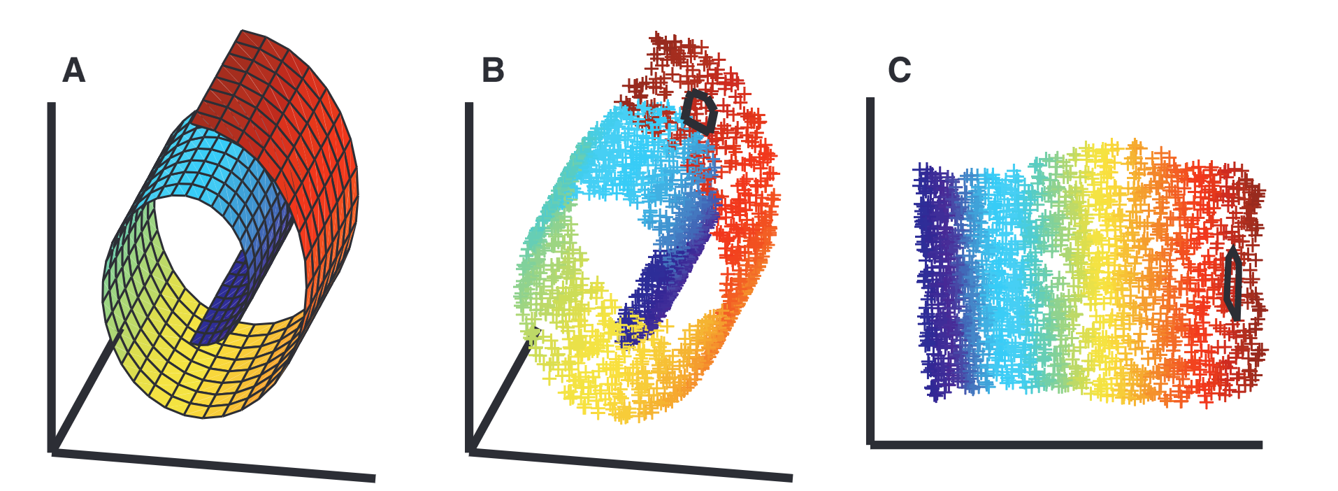
The note is an over-simplified brief about manifold learning in AI.
Source:
Most of the figures in this article are sourced from Yubei Chen's course, EEC289A, at UC Davis.
Source:
Most of the figures in this article are sourced from Yubei Chen's course, EEC289A, at UC Davis.
TL;DR: In a convolution layer, \[ \text { Output size }=\left\lfloor\frac{\text { Input size }+2 \times \text { Padding }- \text { Kernel size }}{\text { Stride }}\right\rfloor+1 \]
Sources:
Source:
【唐】 牛峤
鵁鶄飞起郡城东。碧江空,半滩风。越王宫殿,蘋叶藕花中。帘卷水楼鱼浪起,千片雪,雨蒙蒙。
【五代】 徐昌图
饮散离亭西去,浮生常恨飘蓬。回头烟柳渐重重。淡云孤雁远,寒日暮天红。 今夜画船何处?潮平淮月朦胧。酒醒人静奈愁浓。残灯孤枕梦,轻浪五更风。
【宋】 王沂孙
渐新痕悬柳,淡彩穿花,依约破初暝。便有团圆意,深深拜,相逢谁在香径。画眉未稳。料素娥、犹带离恨。最堪爱、一曲银钩小,宝帘挂秋冷。
千古盈亏休问。叹慢磨玉斧,难补金镜。太液池犹在,凄凉处、何人重赋清景。故山夜永。试待他、窥户端正。看云外山河,还老尽、桂花影。
【宋】 金德淑
春睡起,积雪满燕山。万里长城横缟带,六街灯火已阑珊,人立玉楼间。