DEtection TRansformer (DETR)

Posted on 2025-11-25 Edited on 2026-03-09 In AI Views:

Sources:

DETR paper: End-to-End Object Detection with Transformers

DEtection TRansformer (DETR)

Notation

Symbol	Type	Explanation
\(I\)	Input image	A batch of images, shape \((B, 3, H_{\text{img}}, W_{\text{img}})\)
\(B\)	Batch size	Number of images in a batch
\(F\)	Feature map	Backbone output feature map, shape \((B, D, H_f, W_f)\)
\(D\)	Feature dimension	Channel or embedding dimension (DETR default \(D=256\) after 1×1 conv)
\(H_f, W_f\)	Spatial size	Height/width of backbone feature map
\(HW\)	Token count	Flattened spatial token count, \(HW = H_f \times W_f\)
\(X\)	Image tokens	Flattened feature tokens, shape \((B, HW, D)\)
\(PE\)	Positional encoding	2D positional encoding added to image tokens
\(M\)	Image memory	Encoder output tokens, shape \((B, HW, D)\)
\(N\)	# query slots	Fixed number of object queries or slots (DETR default \(N=100\))
\(Q_0\)	Object queries	Learnable query embeddings, shape \((N, D)\) → broadcast to \((B, N, D)\)
\(Q_L\)	Final query features	Decoder output per-slot features, shape \((B, N, D)\)
\(C\)	# classes	Number of foreground classes (plus one no-object class)
\(\varnothing\)	No-object class	Special class meaning “this slot predicts no object”
\(K\)	# GT objects	Number of ground-truth objects in an image (variable, \(K \le N\))

1. What is DETR?

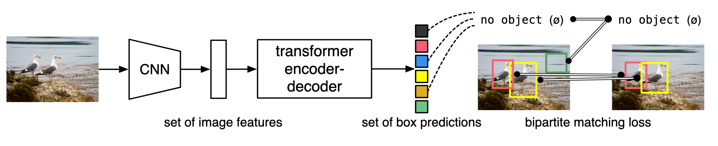
Fig. 1: DETR directly predicts (in parallel) the final set of detections by combining a common CNN with a transformer architecture. During training, bipartite matching uniquely assigns predictions with ground truth boxes. Prediction with no match should yield a “no object” (\(\varnothing\)) class prediction.

DETR is the first clean end-to-end object detector built around a Transformer. Its core idea is simple: Treat object detection as a direct set prediction problem.

Given an image, the model outputs a set of objects in one shot. Each object has:

a class label class
a bounding box box

So DETR does not first generate tons of candidate boxes and then filter/merge them. It predicts the fixed-size final set directly.

DETR achieves this mainly using:

a Transformer encoder–decoder to reason globally and assign objects to slots
a set loss with Hungarian matching to enforce unique, non-duplicated predictions

2. What improves over previous detectors?

A typical traditional detection pipeline looks like:

generate many candidates (anchors/proposals) → classify/regress → NMS to remove duplicates

This pipeline relies on many hand-designed components and heuristics.

DETR simplifies it in three key ways:

No anchors / proposals
- no dense candidate generation
- directly predicts the final object set
No NMS
- deduplication is learned through the set loss + query interactions, not a post-processing step
Fully end-to-end and unified
- training objective matches inference outputs exactly
- the pipeline is conceptually clean

One-liner:

DETR moves detection from dense+heuristic pipelines to set+matching.

3. Components and workflow (including object queries)

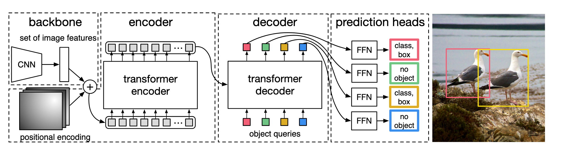
Fig. 2: DETR uses a conventional CNN backbone to learn a 2D representation of an input image. The model flattens it and supplements it with a positional encoding before passing it into a transformer encoder. A transformer decoder then takes as input a small fixed number of learned positional embeddings, which we call object queries, and additionally attends to the encoder output. We pass each output embedding of the decoder to a shared feed forward network (FFN) that predicts either a detection (class and bounding box) or a “no object” class.

3.1 Components

DETR has a very structured three-part design:

Backbone (CNN/ViT)
- extracts an image feature map
Transformer Encoder
- takes only image tokens (with 2D positional encoding)
- outputs a global image memory
Transformer Decoder
- takes a fixed set of object queries (N slots)
- uses attention to read the image memory
- each query outputs either an object prediction or no-object

3.2 Workflow (detailed)

It’s easiest to see DETR as two separate streams: an image stream (encoder path) and a slot/query stream (decoder path). They stay separate until the decoder’s cross-attention.

A. Image stream (goes into the Encoder only)

Step A1: Backbone feature extraction

1 2	Image I → Backbone → Feature map F F shape: (B, D, H_f, W_f)

Typical scale example:

input ~800×800
stride ~32
so H_f≈20, W_f≈20
D=256

Step A2: Flatten into image tokens

1 2	X = flatten(F) X shape: (B, HW, D), HW = H_f × W_f

Example:

H_f=W_f=20 → HW=400
X shape: (B, 400, 256)

Step A3: Add 2D positional encoding (image tokens only)

1 2	X' = X + PE shape unchanged: (B, HW, D)

Step A4: Transformer Encoder (global reasoning)

1 2	M = Encoder(X') M shape: (B, HW, D)

Intuition:

The encoder “reads” the whole image and produces a global memory bank M.

B. Slot / Query stream (goes into the Decoder only)

Step B1: Prepare N object queries (independent learnable slots)

Formally:

1	Q0 = nn.Embedding(N, D)

Example (DETR default):

N=100
D=256
Q0 shape: (100, 256)
broadcast to batch: (B, 100, 256)

Important:

queries are not computed from the image
they never enter the encoder
they are the decoder’s input sequence

Intuition:

These are N empty “slots” the model can fill with objects.

Step B2: Transformer Decoder (where queries meet memory)

Each decoder layer performs:

Self-attention on queries
- (I suppose it) lets slots communicate to avoid duplicate detections
Cross-attention (queries read image memory)
- each slot searches the memory for “its” object
FFN
- refines each slot’s representation

After L layers:

1	QL shape: (B, N, D)

(Optional note for SAM3)

SAM3 uses a DETR-like decoder too: learned queries cross-attend to conditioned image embeddings; prompts just condition the slots before they claim objects.

Step B3: Prediction heads

Per query output:

class logits (including a no-object class)
normalized box (cx, cy, w, h)

1 2	class_logits shape: (B, N, C+1) boxes shape: (B, N, 4)

3.3 What exactly are object queries (slots)?

Object queries are N learnable embeddings. They function as:

N object slots in the decoder.

After training:

some slots align to real objects
remaining slots learn to output no-object (∅)

Intuition:

Give the model N empty seats; it decides which seats correspond to objects and which stay empty.

3.4 Concrete example (to make “N slots” tangible)

Suppose an image contains only 3 objects:

person
dog
ball

So GT count is K=3, but DETR still outputs N=100 slots.

Inference output is always length 100:

1	pred = [(class_1, box_1), ..., (class_100, box_100)]

A typical learned allocation might look like:

slot id	predicted class	meaning
q5	person	slot #5 claims the person
q17	dog	slot #17 claims the dog
q63	ball	slot #63 claims the ball
other 97 slots	no-object (∅)	empty slots

So:

Out of 100 slots, only 3 are “filled” with objects; the rest predict ∅.

4. Training (very short)

Training has two essential steps:

Hungarian matching (1-to-1 assignment)
- match K GT objects to K of the N predicted slots
- remaining N−K slots are matched to ∅
Loss on matched pairs
- matched slots: classification loss + box loss (L1 + GIoU)
- unmatched slots: supervised as no-object (∅)

One-liner:

DETR trains by assigning objects to slots, not by filtering candidates.

Appendix

Box vs. normalized box

A box is an axis-aligned rectangle for an object. DETR predicts normalized boxes, meaning coordinates are scaled to [0, 1] by image width/height, so training is stable and resolution-independent.

DETR uses the center-size format:

[ (cx,, cy,, w,, h) ]

\(cx, cy\): box center (relative to image size)
\(w, h\): box width/height (relative to image size)

Why 4 numbers?

A rectangle needs 4 degrees of freedom: 2 for position + 2 for size. This is equivalent to the corner format \((x_1, y_1, x_2, y_2)\); DETR uses center-size because it’s smooth/easy to regress and avoids constraints like \(x_1 < x_2\).