Actor-Critic Methods
Actor-critic methods are still policy gradient methods. Compared to REINFORCE, actor-critic methods use TD learning to approximate the action value \(q_\pi\left(s_t, a_t\right)\).
What are "actor" and "critic"?
- Here, "actor" refers to policy update. It is called actor is because the policies will be applied to take actions.
- Here, "critic" refers to policy evaluation or value estimation. It is called critic because it criticizes the policy by evaluating it.
Sources:
The simplest actor-critic (QAC)
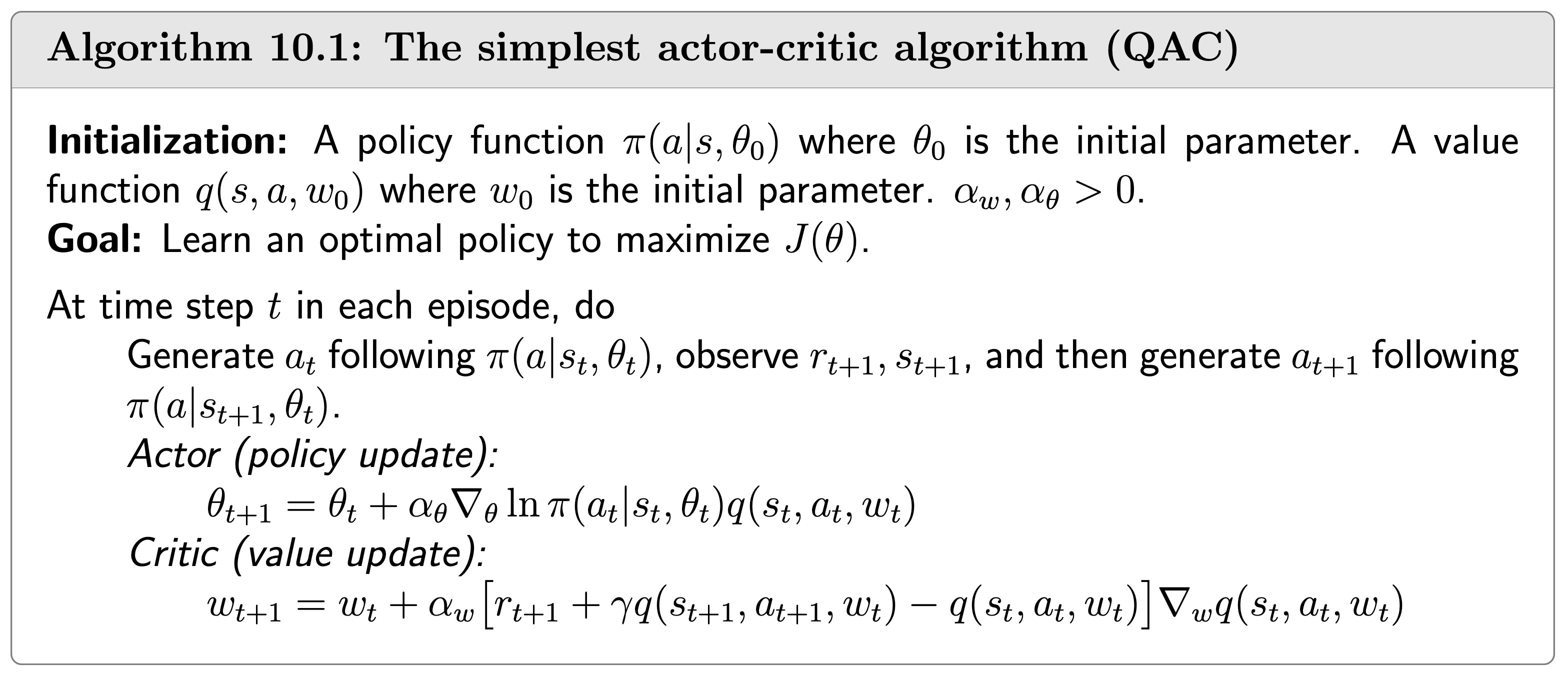
Revisit the idea of policy gradient introduced in the post about policy gradient methods.
A scalar metric \(J(\theta)\), which can be \(\bar{v}_\pi\) or \(\bar{r}_\pi\).
The gradient-ascent algorithm maximizing \(J(\theta)\) is $$ \[\begin{aligned} \theta_{t+1} &= \theta_t+\alpha \color{orange}{\nabla_\theta J (\theta_t )} \\ &= \theta_t+\alpha \color{orange}{\mathbb{E}_{S \sim \eta, A \sim \pi(S, \theta)} [\nabla_{\theta} \ln \pi (A \mid S, \theta_t) q_{\pi}(S, A) ]} \end{aligned}\]$$
The stochastic gradient-ascent algorithm is \[ \theta_{t+1}=\theta_t+\alpha \color{pink}{\nabla_\theta \ln \pi\left(a_t \mid s_t, \theta_t\right) q_\pi\left(s_t, a_t\right)} \] We can see "actor" and "critic" from this algorithm: - This algorithm corresponds to actor. - The algorithm estimating \(q_t(s, a)\) corresponds to critic.
This is the simplest actor-critic method, also called QAC, Q for Q value.
As a policy gradient method, QAC is also on-policy.
Adding baseline functions
Next, we extend QAC to advantage actor-critic (A2C). The core idea is to introduce a "baseline" function, which is a a scalar function of the state random variable \(S\), denoted as \(b(S)\), into the policy gradient \[ \begin{aligned} \nabla_\theta J(\theta) & =\mathbb{E}_{S \sim \eta, A \sim \pi}\left[\nabla_\theta \ln \pi\left(A \mid S, \theta_t\right) q_\pi(S, A)\right] \\ & =\mathbb{E}_{S \sim \eta, A \sim \pi}\left[\nabla_\theta \ln \pi\left(A \mid S, \theta_t\right)\left(q_\pi(S, A)-\color{blue}{b(S)}\right)\right] \end{aligned} \] We can prove that the second equation holds, i.e., the policy gradient \(\nabla_\theta J(\theta)\) is invariant to an additional baseline \(b(S)\).
The purpose of adding this \(b(S)\) is that, if we write \[ \nabla_\theta J(\theta)=\mathbb{E}[X], \] where \[ X(S, A) \doteq \nabla_\theta \ln \pi\left(A \mid S, \theta_t\right)\left[q_\pi(S, A)-b(S)\right], \]
altough \(\mathbb{E}[X]\) is invariant to \(b(S)\), the variance \(\operatorname{var}(X)\) is NOT invariant to \(b(S)\).
This is because \(\operatorname{tr}[\operatorname{var}(X)]=\mathbb{E}\left[X^T X\right]-\bar{x}^T \bar{x}\) and \[ \begin{aligned} \mathbb{E}\left[X^T X\right] & =\mathbb{E}\left[\left(\nabla_\theta \ln \pi\right)^T\left(\nabla_\theta \ln \pi\right)\left(q_\pi(S, A)-b(S)\right)^2\right] \\ & =\mathbb{E}\left[\left\|\nabla_\theta \ln \pi\right\|^2\left(q_\pi(S, A)-b(S)\right)^2\right] \end{aligned} \]
#TODO
Therefore, our goal is to select an optimal baseline \(b\) to minimize \(\operatorname{var}(X)\).
The optimal baseline
The optimal baseline that can minimize \(\operatorname{var}(X)\) is, for any \(s \in \mathcal{S}\), \[ b^*(s) = \frac{\mathbb{E}_{A \sim \pi}\left[ \color{blue}{\left\|\nabla_\theta \ln \pi\left(A \mid s, \theta_t\right)\right\|^2} \color{red}{q_\pi(s, A)}\right]}{\mathbb{E}_{A \sim \pi}\left[\color{blue}{\left\|\nabla_\theta \ln \pi\left(A \mid s, \theta_t\right)\right\|^2}\right]} . \]
See the proof in the appendix.
Advantage actor-critic (A2C)
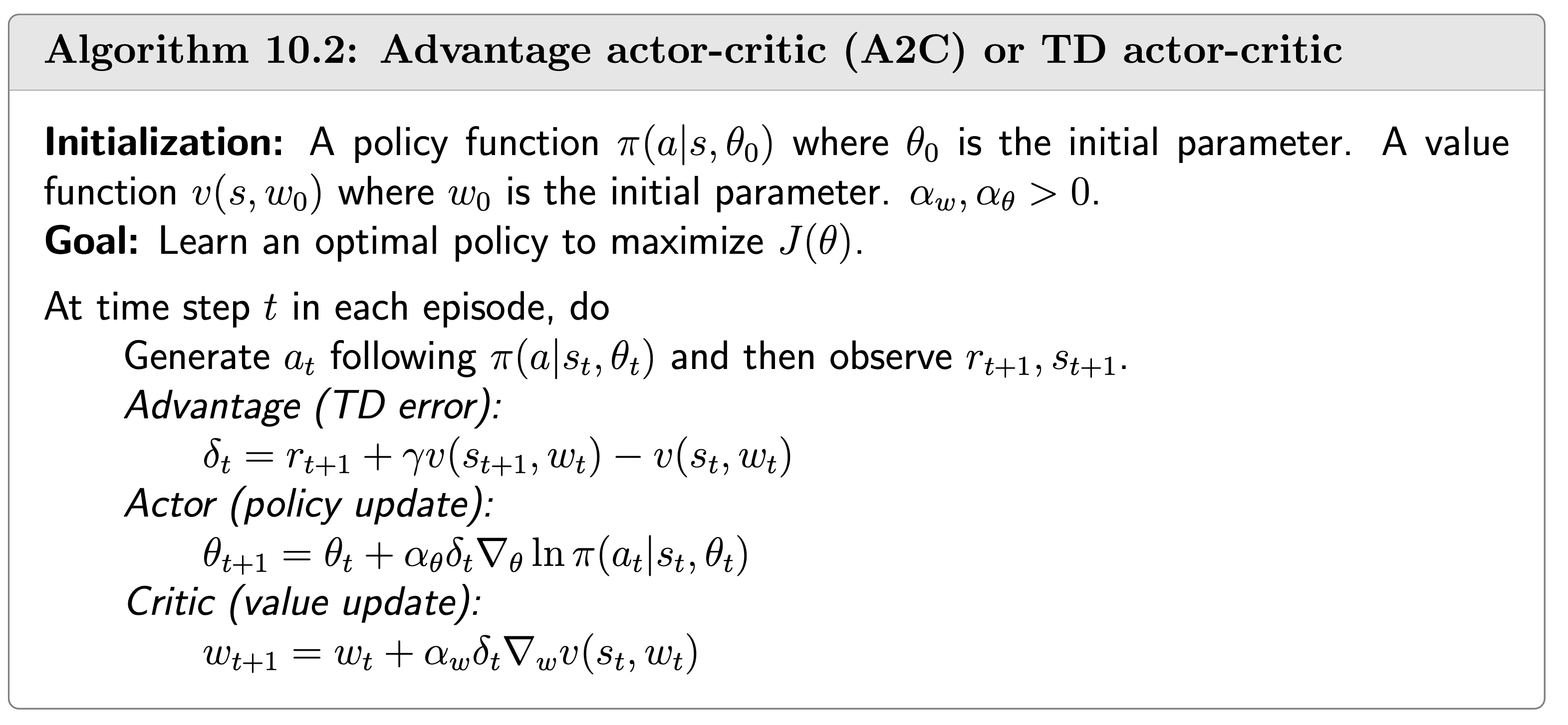
The optimal baseline we introduced is complex. We can remove the weight \(\color{blue}{\left\|\nabla_\theta \ln \pi\left(A \mid s, \theta_t\right)\right\|^2}\) and select the suboptimal baseline: \[ b(s)=\mathbb{E}_{A \sim \pi}\left[q_\pi(s, A)\right]=v_\pi(s) \] which is the state value of \(s\).
Now we let \(b(s)=v_\pi(s)\), the policy gradient becomes \[ \begin{aligned} \nabla_\theta J(\theta) & =\mathbb{E}_{S \sim \eta, A \sim \pi}\left[\nabla_\theta \ln \pi\left(A \mid S, \theta_t\right) q_\pi(S, A)\right] \\ & =\mathbb{E}_{S \sim \eta, A \sim \pi}\left[\nabla_\theta \ln \pi\left(A \mid S, \theta_t\right)\left(q_\pi(S, A)-\color{blue}{v_{\pi}(S)}\right)\right] \\ & =\mathbb{E}_{S \sim \eta, A \sim \pi}\left[\nabla_\theta \ln \pi\left(A \mid S, \theta_t\right)\color{purple}{\delta_\pi(S, A)}\right] \end{aligned} \] where \[ \delta_\pi(S, A) \doteq q_\pi(S, A)-v_\pi(S) \] is called the advantage function.
The stochastic gradient optimization process is \[ \begin{aligned} \theta_{t+1} & =\theta_t+\alpha \nabla_\theta \ln \pi\left(a_t \mid s_t, \theta_t\right)\left[q_t\left(s_t, a_t\right)-v_t\left(s_t\right)\right] \\ & =\theta_t+\alpha \nabla_\theta \ln \pi\left(a_t \mid s_t, \theta_t\right) \delta_t\left(s_t, a_t\right) \end{aligned} \]
Off-policy actor-critic
Appendix
Proof of baseline invariance
We need to prove \[ \mathbb{E}_{S \sim \eta, A \sim \pi}\left[\nabla_\theta \ln \pi\left(A \mid S, \theta_t\right) b(S)\right]=0 \]
The details: \[ \begin{aligned} \mathbb{E}_{S \sim \eta, A \sim \pi}\left[\nabla_\theta \ln \pi\left(A \mid S, \theta_t\right) b(S)\right] & =\sum_{s \in \mathcal{S}} \eta(s) \sum_{a \in \mathcal{A}} \pi\left(a \mid s, \theta_t\right) \nabla_\theta \ln \pi\left(a \mid s, \theta_t\right) b(s) \\ & =\sum_{s \in \mathcal{S}} \eta(s) \sum_{a \in \mathcal{A}} \nabla_\theta \pi\left(a \mid s, \theta_t\right) b(s) \\ & =\sum_{s \in \mathcal{S}} \eta(s) b(s) \sum_{a \in \mathcal{A}} \nabla_\theta \pi\left(a \mid s, \theta_t\right) \\ & =\sum_{s \in \mathcal{S}} \eta(s) b(s) \nabla_\theta \sum_{a \in \mathcal{A}} \pi\left(a \mid s, \theta_t\right) \\ & =\sum_{s \in \mathcal{S}} \eta(s) b(s) \nabla_\theta 1=0 \end{aligned} \]
Showing that \(b^*(s)\) is the optimal baseline
Let \(\bar{x} \doteq \mathbb{E}[X]\), which is invariant for any \(b(s)\). If \(X\) is a vector, its variance is a matrix. It is common to select the trace of \(\operatorname{var}(X)\) as a scalar objective function for optimization: \[ \begin{aligned} \operatorname{tr}[\operatorname{var}(X)] & =\operatorname{tr} \mathbb{E}\left[(X-\bar{x})(X-\bar{x})^T\right] \\ & =\operatorname{tr} \mathbb{E}\left[X X^T-\bar{x} X^T-X \bar{x}^T+\bar{x} \bar{x}^T\right] \\ & =\operatorname{tr} \mathbb{E}\left[X X^T-\bar{x} X^T-X \bar{x}^T+\bar{x} \bar{x}^T\right] \\ & =\mathbb{E}\left[X^T X-X^T \bar{x}-\bar{x}^T X+\bar{x}^T \bar{x}\right] \\ & =\mathbb{E}\left[X^T X\right]-\bar{x}^T \bar{x} . \end{aligned} \]
When deriving the above equation, we use the trace property \(\operatorname{tr}(A B)=\operatorname{tr}(B A)\) for any squared matrices \(A, B\) with appropriate dimensions. Since \(\bar{x}\) is invariant, equation \[ \mathbb{E}\left[X^T X\right]-\bar{x}^T \bar{x} \] suggests that we only need to minimize \(\mathbb{E}\left[X^T X\right]\). With \(X\) defined in \[ X(S, A) \doteq \nabla_\theta \ln \pi\left(A \mid S, \theta_t\right)\left[q_\pi(S, A)-b(S)\right], \] we have \[ \begin{aligned} \mathbb{E}\left[X^T X\right] & =\mathbb{E}\left[\left(\nabla_\theta \ln \pi\right)^T\left(\nabla_\theta \ln \pi\right)\left(q_\pi(S, A)-b(S)\right)^2\right] \\ & =\mathbb{E}\left[\left\|\nabla_\theta \ln \pi\right\|^2\left(q_\pi(S, A)-b(S)\right)^2\right], \end{aligned} \] where \(\pi(A \mid S, \theta)\) is written as \(\pi\) for short. Since \(S \sim \eta\) and \(A \sim \pi\), the above equation can be rewritten as \[ \mathbb{E}\left[X^T X\right]=\sum_{s \in \mathcal{S}} \eta(s) \mathbb{E}_{A \sim \pi}\left[\left\|\nabla_\theta \ln \pi\right\|^2\left(q_\pi(s, A)-b(s)\right)^2\right] . \]
To ensure \(\nabla_b \mathbb{E}\left[X^T X\right]=0, b(s)\) for any \(s \in \mathcal{S}\) should satisfy \[ \mathbb{E}_{A \sim \pi}\left[\left\|\nabla_\theta \ln \pi\right\|^2\left(b(s)-q_\pi(s, A)\right)\right]=0, \quad s \in \mathcal{S} . \]
The above equation can be easily solved to obtain the optimal baseline: \[ b^*(s)=\frac{\mathbb{E}_{A \sim \pi[}\left[\left\|\nabla_\theta \ln \pi\right\|^2 q_\pi(s, A)\right]}{\mathbb{E}_{A \sim \pi}\left[\left\|\nabla_\theta \ln \pi\right\|^2\right]}, \quad s \in \mathcal{S} . \]