Off-Policy Actor-Critic Methods

Posted on 2024-06-24 Edited on 2024-09-17 In Computer Science Views:

The policy gradient methods that we have studied so far, including REINFORCE, QAC, and $\mathrm{A} 2 \mathrm{C}$, are all on-policy. The reason for this can be seen from the expression of the true gradient: \[ \nabla_\theta J(\theta)=\mathbb{E}_{S \sim \eta, A \sim \pi}\left[\nabla_\theta \ln \pi\left(A \mid S, \theta_t\right)\left(q_\pi(S, A)-v_\pi(S)\right)\right] . \]

To use samples to approximate this true gradient, we must generate the action samples by following $\pi(\theta)$. Hence, $\pi(\theta)$ is the behavior policy. Since $\pi(\theta)$ is also the target policy that we aim to improve, the policy gradient methods are on-policy.

In the case that we already have some samples generated by a given behavior policy, the policy gradient methods can still be applied to utilize these samples. To do that, we can employ a technique called importance sampling. It is a general technique for estimating expected values defined over one probability distribution using some samples drawn from another distribution.

Sources:

Shiyu Zhao. Chapter 10: Actor-Critic Methods. Mathematical Foundations of Reinforcement Learning.

Importance sampling

We next introduce the importance sampling technique. Consider a random variable $X \in \mathcal{X}$. Suppose that $p_0(X)$ is a probability distribution. Our goal is to estimate $\mathbb{E}_{X \sim p_0}[X]$. Suppose that we have some i.i.d. samples $\left\{x_i\right\}_{i=1}^n$.

Suppose the samples $\left\{x_i\right\}_{i=1}^n$ are not generated by $p_0$. Instead, they are generated by another distribution $p_1$. Can we still use these samples to approximate $\mathbb{E}_{X \sim p_0}[X]$ ? The answer is yes. $\mathbb{E}_{X \sim p_0}[X]$ can be approximated based on the importance sampling technique.

In particular, $\mathbb{E}_{X \sim p_0}[X]$ satisfies \[ \mathbb{E}_{X \sim p_0}[X]=\sum_{x \in \mathcal{X}} p_0(x) x=\sum_{x \in \mathcal{X}} p_1(x) \underbrace{\frac{p_0(x)}{p_1(x)} x}_{f(x)}= \color{teal}{\mathbb{E}_{X \sim p_1}[f(X)]} . \]

Thus, estimating $\mathbb{E}_{X \sim p_0}[X]$ becomes the problem of estimating $\mathbb{E}_{X \sim p_1}[f(X)]$. Let \[ \bar{f} \doteq \frac{1}{n} \sum_{i=1}^n f\left(x_i\right) \]

Since $\bar{f}$ can effectively approximate $\mathbb{E}_{X \sim p_1}[f(X)]$, we obtain \[ \mathbb{E}_{X \sim p_0}[X]=\color{teal}{\mathbb{E}_{X \sim p_1}[f(X)]} \approx \bar{f}=\frac{1}{n} \sum_{i=1}^n f\left(x_i\right)=\frac{1}{n} \sum_{i=1}^n \underbrace{\frac{p_0\left(x_i\right)}{p_1\left(x_i\right)}}_{\begin{array}{c} \text { importance } \\ \text { weight } \end{array}} x_i . \]

Here, $\frac{p_0\left(x_i\right)}{p_1\left(x_i\right)}$ is called the importance weight. When $p_1=p_0$, the importance weight is 1 and $\bar{f}$ becomes $\bar{x}$. When $p_0\left(x_i\right) \geq p_1\left(x_i\right), x_i$ can be sampled more frequently by $p_0$ but less frequently by $p_1$. In this case, the importance weight, which is greater than one, emphasizes the importance of this sample.

You may ask that while $p_0(x)$ is required in \[ \begin{equation} \label{eq10_10} \frac{1}{n} \sum_{i=1}^n \frac{p_0\left(x_i\right)}{p_1\left(x_i\right)} x_i, \end{equation} \] why do we not directly calculate $\mathbb{E}_{X \sim p_0}[X]$ using its definition \[ \mathbb{E}_{X \sim p_0}[X]=\sum_{x \in \mathcal{X}} p_0(x) x \] ?

The answer is as follows. To use the definition, we need to know either the analytical expression of $p_0$ or the value of $p_0(x)$ for every $x \in \mathcal{X}$. However, it is difficult to obtain the analytical expression of $p_0$ when the distribution is represented by, for example, a neural network. It is also difficult to obtain the value of $p_0(x)$ for every $x \in \mathcal{X}$ when $\mathcal{X}$ is large. By contrast, $\eqref{eq10_10}$ merely requires the values of $p_0\left(x_i\right)$ for some samples and is much easier to implement in practice.

The off-policy policy gradient theorem

Like the previous on-policy case, we need to derive the policy gradient in the off-policy case.

Suppose $\beta$ is the behavior policy that generates experience samples.
Our aim is to use these samples to update a target policy $\pi$ that can minimize the metric \[ J(\theta)=\sum_{s \in \mathcal{S}} d_\beta(s) v_\pi(s)=\mathbb{E}_{S \sim d_\beta}\left[v_\pi(S)\right] \] where $d_\beta$ is the stationary distribution under policy $\beta$ and $v_\pi$ is the state value under policy $\pi$.

The gradient of this metric is given in the following theorem.

Theorem 10.1 (Off-policy policy gradient theorem). In the discounted case where $\gamma \in$ $(0,1)$, the gradient of $J(\theta)$ is \[ \nabla_\theta J(\theta)=\mathbb{E}_{S \sim \rho, A \sim \beta}[\underbrace{\frac{\pi(A \mid S, \theta)}{\beta(A \mid S)}}_{\begin{array}{c} \text { importance } \\ \text { weight } \end{array}} \nabla_\theta \ln \pi(A \mid S, \theta) q_\pi(S, A)], \] where the state distribution $\rho$ is \[ \rho(s) \doteq \sum_{s^{\prime} \in \mathcal{S}} d_\beta\left(s^{\prime}\right) \operatorname{Pr}_\pi\left(s \mid s^{\prime}\right), \quad s \in \mathcal{S}, \] where \[ \operatorname{Pr}_\pi\left(s \mid s^{\prime}\right)=\sum_{k=0}^{\infty} \gamma^k\left[P_\pi^k\right]_{s^{\prime} s}=\left[\left(I-\gamma P_\pi\right)^{-1}\right]_{s^{\prime} s} \] is the discounted total probability of transitioning from $s^{\prime}$ to $s$ under policy $\pi$.

The gradient $\nabla_\theta J(\theta)$ is similar to that in the on-policy case in Theorem 9.1, but there are two differences. The first difference is the importance weight. The second difference is that $A \sim \beta$ instead of $A \sim \pi$. Therefore, we can use the action samples generated by following $\beta$ to approximate the true gradient. The proof of the theorem is given in the appendix.

The off-policy policy gradient is also invariant to a baseline $b(s)$. In particular, we have

\[ \nabla_\theta J(\theta)=\mathbb{E}_{S \sim \rho, A \sim \beta}\left[\frac{\pi(A \mid S, \theta)}{\beta(A \mid S)} \nabla_\theta \ln \pi(A \mid S, \theta)\left(q_\pi(S, A)-\color{blue}{b(S)}\right)\right] \] because \[ \mathbb{E}\left[\frac{\pi(A \mid S, \theta)}{\beta(A \mid S)} \nabla_\theta \ln \pi(A \mid S, \theta) b(S)\right]=0 . \]

To reduce the estimation variance, we select the baseline as $b(S)=v_\pi(S)$ as in A2C and obtain \[ \nabla_\theta J(\theta)=\mathbb{E}\left[\frac{\pi(A \mid S, \theta)}{\beta(A \mid S)} \nabla_\theta \ln \pi(A \mid S, \theta)\left(q_\pi(S, A)-\color{blue}{v_\pi(S)}\right)\right] \]

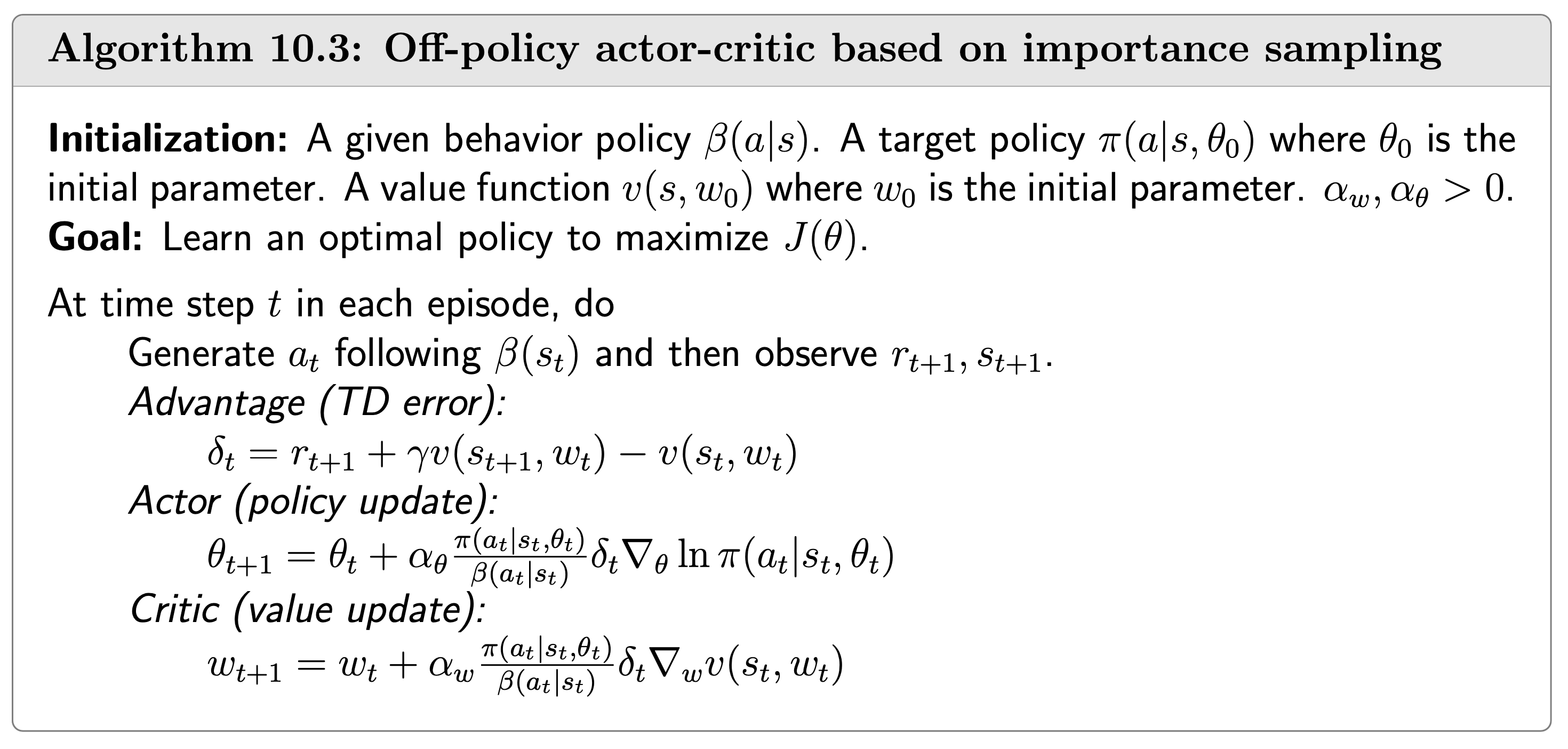
The corresponding stochastic gradient-ascent algorithm is \[ \theta_{t+1}=\theta_t+\alpha_\theta \frac{\pi\left(a_t \mid s_t, \theta_t\right)}{\beta\left(a_t \mid s_t\right)} \nabla_\theta \ln \pi\left(a_t \mid s_t, \theta_t\right)\left(q_t\left(s_t, a_t\right)-v_t\left(s_t\right)\right) \]

Similar to the on-policy case, \[ q_t\left(s_t, a_t\right)-v_t\left(s_t\right) \approx r_{t+1}+\gamma v_t\left(s_{t+1}\right)-v_t\left(s_t\right) \doteq \delta_t\left(s_t, a_t\right) \]

Then, the algorithm becomes \[ \theta_{t+1}=\theta_t+\alpha_\theta \frac{\pi\left(a_t \mid s_t, \theta_t\right)}{\beta\left(a_t \mid s_t\right)} \nabla_\theta \ln \pi\left(a_t \mid s_t, \theta_t\right) \delta_t\left(s_t, a_t\right) \] and hence \[ \theta_{t+1}=\theta_t+\alpha_\theta\left(\frac{\delta_t\left(s_t, a_t\right)}{\beta\left(a_t \mid s_t\right)}\right) \nabla_\theta \pi\left(a_t \mid s_t, \theta_t\right) \]

Appendix

Proof of Theorem 10.1

Since $d_\beta$ is independent of $\theta$, the gradient of $J(\theta)$ satisfies \[ \nabla_\theta J(\theta)=\nabla_\theta \sum_{s \in \mathcal{S}} d_\beta(s) v_\pi(s)=\sum_{s \in \mathcal{S}} d_\beta(s) \nabla_\theta v_\pi(s) . \]

According to Lemma 9.2, the expression of $\nabla_\theta v_\pi(s)$ is \[ \color{salmon}{\nabla_\theta v_\pi(s)=\sum_{s^{\prime} \in \mathcal{S}} \operatorname{Pr}_\pi\left(s^{\prime} \mid s\right) \sum_{a \in \mathcal{A}} \nabla_\theta \pi\left(a \mid s^{\prime}, \theta\right) q_\pi\left(s^{\prime}, a\right)}, \] where \[ \operatorname{Pr}_\pi\left(s^{\prime} \mid s\right) \doteq \sum_{k=0}^{\infty} \gamma^k\left[P_\pi^k\right]_{s s^{\prime}}=\left[\left(I_n-\gamma P_\pi\right)^{-1}\right]_{s s^{\prime}} \] Substituting $\color{salmon}{\nabla_\theta v_\pi(s)}$ into $\sum_{s \in \mathcal{S}} d_\beta(s) \nabla_\theta v_\pi(s)$ yields \[ \begin{aligned} \nabla_\theta J(\theta)=\sum_{s \in \mathcal{S}} d_\beta(s) \nabla_\theta v_\pi(s) & =\sum_{s \in \mathcal{S}} d_\beta(s) \sum_{s^{\prime} \in \mathcal{S}} \operatorname{Pr}_\pi\left(s^{\prime} \mid s\right) \sum_{a \in \mathcal{A}} \nabla_\theta \pi\left(a \mid s^{\prime}, \theta\right) q_\pi\left(s^{\prime}, a\right) \\ & =\sum_{s^{\prime} \in \mathcal{S}}\left(\sum_{s \in \mathcal{S}} d_\beta(s) \operatorname{Pr}_\pi\left(s^{\prime} \mid s\right)\right) \sum_{a \in \mathcal{A}} \nabla_\theta \pi\left(a \mid s^{\prime}, \theta\right) q_\pi\left(s^{\prime}, a\right) \\ & \doteq \sum_{s^{\prime} \in \mathcal{S}} \rho\left(s^{\prime}\right) \sum_{a \in \mathcal{A}} \nabla_\theta \pi\left(a \mid s^{\prime}, \theta\right) q_\pi\left(s^{\prime}, a\right) \\ & =\sum_{s \in \mathcal{S}} \rho(s) \sum_{a \in \mathcal{A}} \nabla_\theta \pi(a \mid s, \theta) q_\pi(s, a) \quad \text { (change } s^{\prime} \text { to } s \text { ) } \\ & =\mathbb{E}_{S \sim \rho}\left[\sum_{a \in \mathcal{A}} \nabla_\theta \pi(a \mid S, \theta) q_\pi(S, a)\right] , \end{aligned} \]

where the 3rd equation is because \[ \rho(s) \doteq \sum_{s^{\prime} \in \mathcal{S}} d_\beta\left(s^{\prime}\right) \operatorname{Pr}_\pi\left(s \mid s^{\prime}\right), \quad s \in \mathcal{S} . \]

By using the importance sampling technique, the above equation can be further rewritten as $$ \[\begin{aligned} \mathbb{E}_{S \sim \rho}\left[\sum_{a \in \mathcal{A}} \nabla_\theta \pi(a \mid S, \theta) q_\pi(S, a)\right] & = \mathbb{E}_{S \sim \rho}\left[\sum_{a \in \mathcal{A}} \color{brown}{\beta(a \mid S)} \frac{\color{silver}{\pi(a \mid S, \theta)}}{\color{brown}{\beta(a \mid S)}} \frac{\nabla_\theta \color{silver}{\pi(a \mid S, \theta)}}{\pi(a \mid S, \theta)} q_\pi(S, a)\right] \\ & =\mathbb{E}_{S \sim \rho}\left[\sum_{a \in \mathcal{A}} \beta(a \mid S) \frac{\pi(a \mid S, \theta)}{\beta(a \mid S)} \nabla_\theta \ln \pi(a \mid S, \theta) q_\pi(S, a)\right] \\ & =\mathbb{E}_{S \sim \rho, A \sim \beta}\left[\frac{\pi(A \mid S, \theta)}{\beta(A \mid S)} \nabla_\theta \ln \pi(A \mid S, \theta) q_\pi(S, A)\right] . \end{aligned}\]

The proof is complete. The above proof is similar to that of Theorem 9.1.