Value Function Approximation
In the previous post, we introduced TD learning algorithms. At that time, all state/action values were represented by tables. This is inefficient for handling large state or action spaces.
In this post, we will use the function approximation method for TD learning. It is also where artificial neural networks are incorporated into reinforcement learning as function approximators.
Sources:
TD learning with function approximation
With function approximation methods, the goal of TD learning is equivalent to is finding the best \(w\) that can minimize the loss function \(J(w)\) \[ \begin{equation} \label{eq1} J(w)=\mathbb{E}_{s \in \mathcal{S}}\left[\left(v_\pi(S)-\hat{v}(S, w)\right)^2\right] \end{equation} \] # Stationary distribution
The expectation in \(\eqref{eq1}\) is with respect to the random variable \(S \in \mathcal{S}\). There are several ways to define the probability distribution of \(S\).
In reinforcement learning (RL), we commonly use the stationary distribution of \(S\) as the distribution of \(S\).
The stationary distribution of \(S\) under policy \(\pi\) can bedenoted by \(\left\{d_\pi(s)\right\}_{s \in \mathcal{S}}\). By definition, \(d_\pi(s) \geq 0\) and \(\sum_{s \in \mathcal{S}} d_\pi(s)=1\).
Let \(n_\pi(s)\) denote the number of times that \(s\) has been visited in a very ong episode generated by \(\pi\). Then, \(d_\pi(s)\) can be approximated by \[ d_\pi(s) \approx \frac{n_\pi(s)}{\sum_{s^{\prime} \in \mathcal{S}} n_\pi\left(s^{\prime}\right)} \] Meanwhile, the converged values \(d_\pi(s)\) can be computed directly by solving equation: \[ d_\pi^T=d_\pi^T P_\pi, \] i.e., \(d_\pi\) is the left eigenvector of \(P_\pi\) associated with the eigenvalue 1. The proof is here.
Optimization algorithms
The loss function \(\eqref{eq1}\) can be rewritten as \[ J(w)=\mathbb{E}\left[\left(v_\pi(S)-\hat{v}(S, w)\right)^2\right]=\sum_{s \in \mathcal{S}} d_\pi(s)\left(v_\pi(s)-\hat{v}(s, w)\right)^2 \]
While we have the objective function, the next step is to optimize it.
To minimize \(J(w)\), we can use the gradient-descent algorithm: \[ w_{k+1}=w_k-\alpha_k \nabla_w J\left(w_k\right) \]
The true gradient is \[ \begin{aligned} \nabla_w J(w) & =\nabla_w \mathbb{E}\left[\left(v_\pi(S)-\hat{v}(S, w)\right)^2\right] \\ & =\mathbb{E}\left[\nabla_w\left(v_\pi(S)-\hat{v}(S, w)\right)^2\right] \\ & =2 \mathbb{E}\left[\left(v_\pi(S)-\hat{v}(S, w)\right)\left(-\nabla_w \hat{v}(S, w)\right)\right] \\ & =-2 \mathbb{E}\left[\left(v_\pi(S)-\hat{v}(S, w)\right) \nabla_w \hat{v}(S, w)\right] \end{aligned} \]
The true gradient above involves the calculation of an expectation. We can use the stochastic gradient to replace the true gradient: \[ w_{t+1}=w_t+\alpha_t\left(\color{teal}{v_\pi\left(s_t\right)}-\hat{v}\left(s_t, w_t\right)\right) \nabla_w \hat{v}\left(s_t, w_t\right) \] where \(s_t\) is a sample of \(S\). Here, \(2 \alpha_k\) is merged to \(\alpha_k\). - This algorithm is not implementable because it requires the true state value \(v_\pi\), which is the unknown to be estimated. - We can replace \(v_\pi\left(s_t\right)\) with an approximation so that the algorithm is implementable.
In particular, - First, Monte Carlo learning with function approximation: Let \(g_t\) be the discounted return starting from \(s_t\) in the episode. Then, \(g_t\) can be used to approximate \(v_\pi\left(s_t\right)\). The algorithm becomes \[ w_{t+1}=w_t+\alpha_t\left(g_t-\hat{v}\left(s_t, w_t\right)\right) \nabla_w \hat{v}\left(s_t, w_t\right) \] - Second, TD learning with function approximation: By the spirit of TD learning, we can replace \(\color{teal}{v_\pi\left(s_t\right)}\) with \(\color{teal}{r_{t+1}+\gamma \hat{v}\left(s_{t+1}, w_t\right)}\). Please remember this substitution is not rigorous. The reason is omitted for simplicity.
After all, the algorithm becomes \[ w_{t+1}=w_t+\alpha_t\left[\color{teal}{r_{t+1}+\gamma \hat{v}\left(s_{t+1}, w_t\right)}-\hat{v}\left(s_t, w_t\right)\right] \nabla_w \hat{v}\left(s_t, w_t\right) \]
Therefore, we can solve TD learning problems[^1] with the function approximation method.
TD learning of action values based on function approximation
Sarsa with function approximation
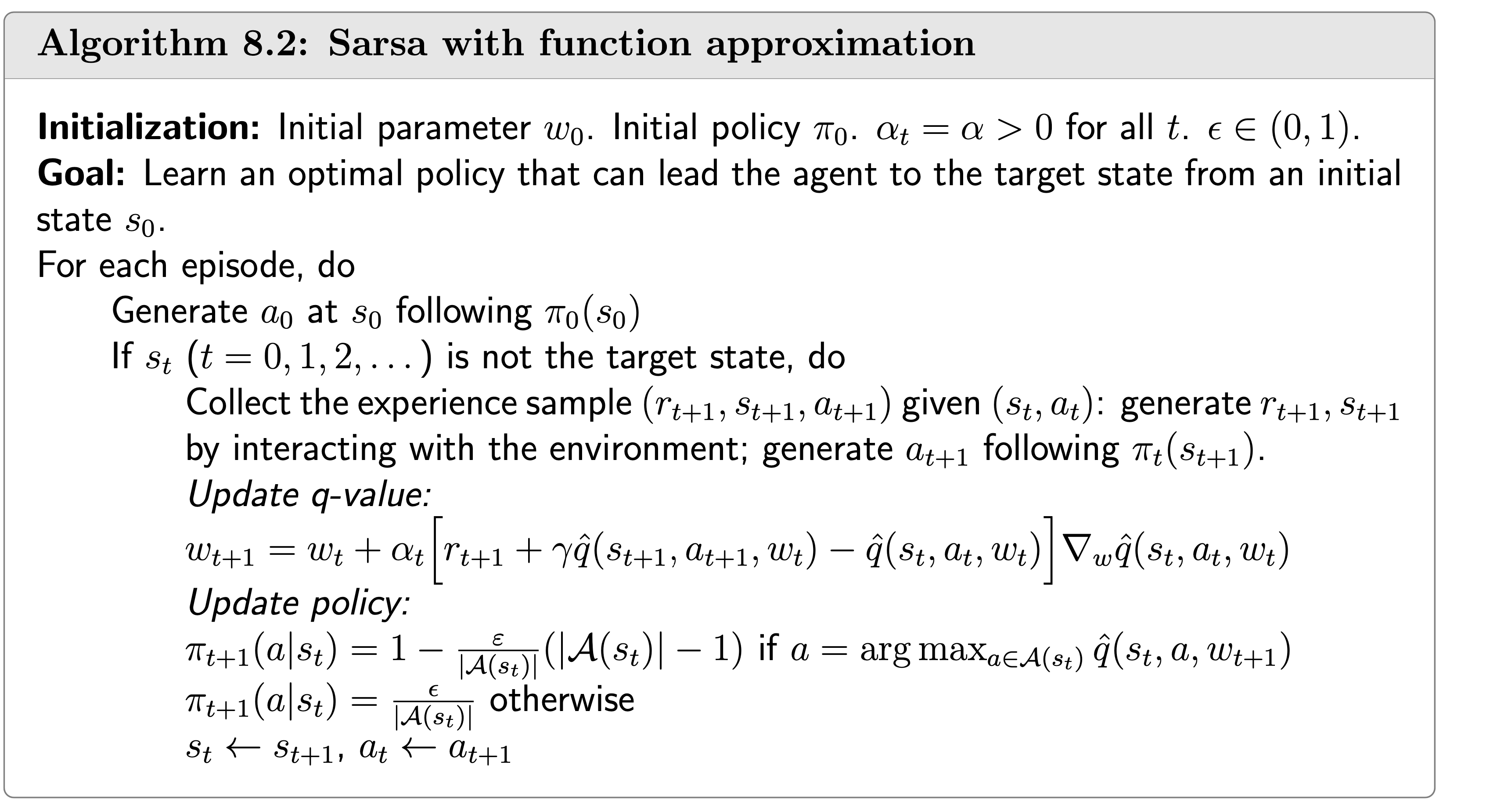
Suppose that \(q_\pi(s, a)\) is approximated by \(\hat{q}(s, a, w)\). Replacing \(\color{brown}{\hat{v}(s, w)}\) in \[ w_{t+1}=w_t+\alpha_t\left[r_{t+1}+\gamma \hat{v}\left(s_{t+1}, w_t\right)-\color{brown}{\hat{v}\left(s_t, w_t\right)}\right] \nabla_w \hat{v}\left(s_t, w_t\right) \] by \(\color{brown}{\hat{q}(s, a, w)}\) gives \[ w_{t+1}=w_t+\alpha_t\left[r_{t+1}+\gamma \hat{q}\left(s_{t+1}, a_{t+1}, w_t\right)-\color{brown}{\hat{q}\left(s_t, a_t, w_t\right)}\right] \nabla_w \hat{q}\left(s_t, a_t, w_t\right) . \]
Q-learning with function approximation
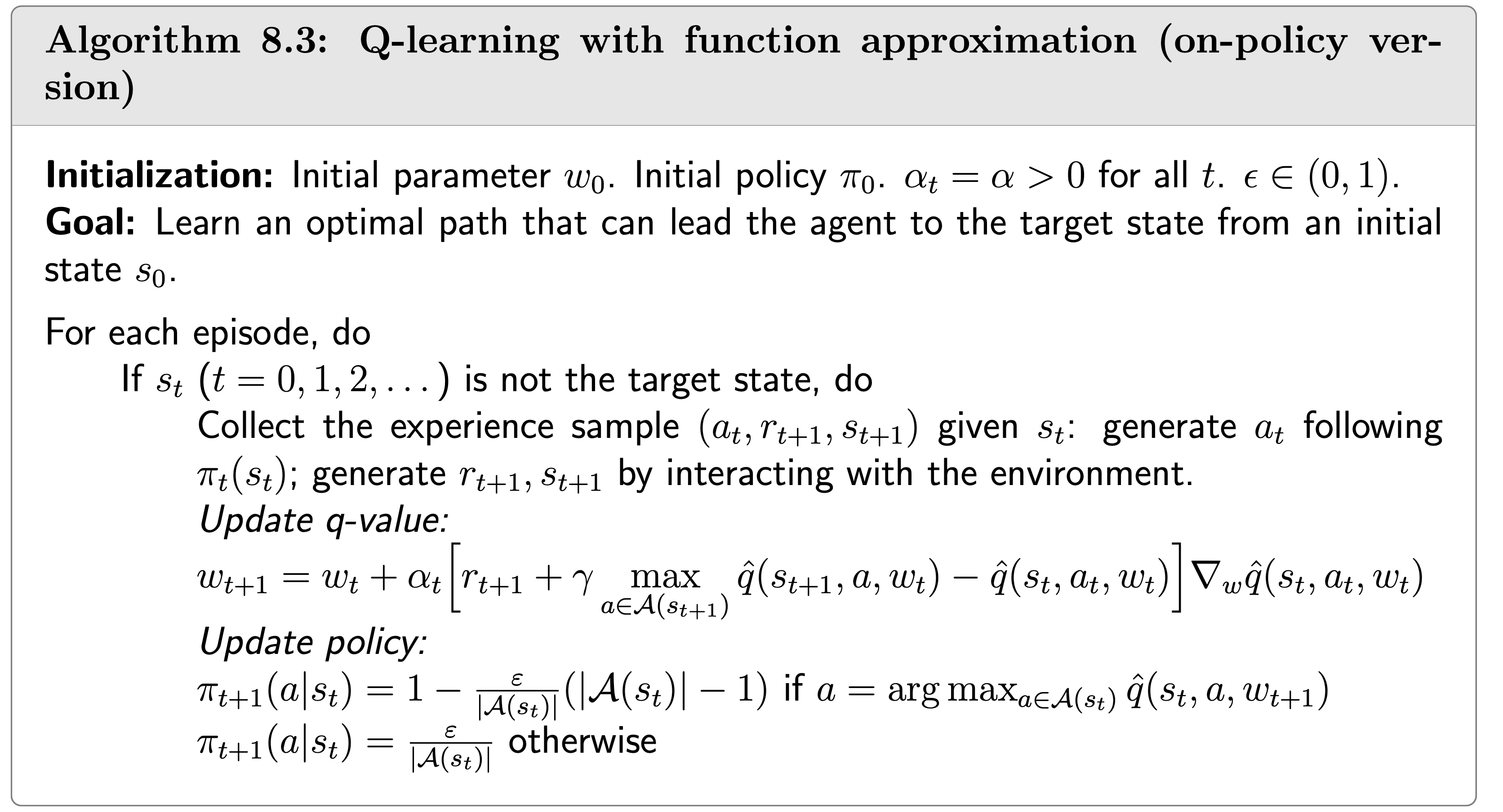
Tabular Q-learning can also be extended to the case of function approximation. The update rule is \[ w_{t+1}=w_t+\alpha_t\left[r_{t+1}+\gamma \color{orange}{\max _{a \in \mathcal{A}\left(s_{t+1}\right)} \hat{q}\left(s_{t+1}, a, w_t\right)}-\hat{q}\left(s_t, a_t, w_t\right)\right] \nabla_w \hat{q}\left(s_t, a_t, w_t\right) . \]
Here, the function approximator is \(\color{teal}{r_{t+1}+\gamma} \color{orange}{\max _{a \in \mathcal{A}\left(s_{t+1}\right)} \hat{q}\left(s_{t+1}, a, w_t\right)}\). It's similar to Sarsa with function approximation except that \(\color{orange}{\hat{q}\left(s_{t+1}, a_{t+1}, w_t\right)}\) is replaced with \(\color{orange}{\max _{a \in \mathcal{A}\left(s_{t+1}\right)} \hat{q}\left(s_{t+1}, a, w_t\right)}\).
NOTE: altough Q-learning with function approximation can be implemented by neural networks. In practice, we choose to use, instead of this method, Deep Q-learning or deep Q-network (DQN). DQN is not Q learning, at least not the specific Q learning algorithm introduced in my post, but it shares the core idea of Q learning.
1 "TD learning problems" refer to the problems aimed to solve by TD learning algorithms, i.e., the state/action value function estimation given a dataset generated by a given policy \(\pi\).