Temporal-Difference Methods

This chapter introduces temporal-difference (TD) methods for reinforcement learning. Similar to Monte Carlo (MC) learning, TD learning is also model-free, but it has some advantages due to its incremental form.

The goal of TD both learning and MC learning is policy evaluation : given a dataset generated by a policy $\pi$, estimate the state value (or action value) of the policy $\pi$. They must be combined with one step of policy improvement to get optimal policies.

We elaborate two TD learning methods: one for estimating state values and one for estimating actions values, the latter algorithm is called Sarsa.

In next post, we will introduce Q-learning, which is very similar to Sarsa, to directly estimate optimal action values and hence optimal policies.

Sources:

1. Shiyu Zhao. Chapter 7: Temporal-Difference Methods. Mathematical Foundations of Reinforcement Learning.

Motivitating examples

Using the RM algorithm to do mean estimations

We next first some stochastic problems and show how to use the RM algorithm to solve them.

First, consider the simple mean estimation problem: calculate $$w=\mathbb{E}[X]$$ based on some iid samples $\{x\}$ of $X$. - By writing $g(w)=w-\mathbb{E}[X]$, we can reformulate the problem to a root-finding problem $$g(w)=0$$ - Since we can only obtain samples $\{x\}$ of $X$, the noisy observation is $$\tilde{g}(w,\eta )=w-x=(w-\mathbb{E}[X])+(\mathbb{E}[X]-x)\doteq g(w)+\eta \text{. }$$ - Then, according to the last lecture, we know the RM algorithm for solving $g(w)=0$ is

$$w_{k+1}=w_k-{\alpha }_k\tilde{g}(w_k,{\eta }_k)=w_k-{\alpha }_k(w_k-x_k)$$

---

Second, consider a little more complex problem. That is to estimate the mean of a function $v(X)$, $$w=\mathbb{E}[v(X)]$$ based on some iid random samples $\{x\}$ of $X$. - To solve this problem, we define $$\begin{array}{rl}g(w)& =w-\mathbb{E}[v(X)]\\ \tilde{g}(w,\eta )& =w-v(x)=(w-\mathbb{E}[v(X)])+(\mathbb{E}[v(X)]-v(x))\doteq g(w)+\eta \end{array}$$ - Then, the problem becomes a root-finding problem: $g(w)=0$. The corresponding RM algorithm is

$$w_{k+1}=w_k-{\alpha }_k\tilde{g}(w_k,{\eta }_k)=w_k-{\alpha }_k[w_k-v\left(x_k\right)]$$

---

Third, consider an even more complex problem: calculate $$w=\mathbb{E}[R+\gamma v(X)]$$ where $R,X$ are random variables, $\gamma$ is a constant, and $v(\cdot )$ is a function. - Suppose we can obtain samples $\{x\}$ and $\{r\}$ of $X$ and $R$. we define $$\begin{array}{rl}g(w)& =w-\mathbb{E}[R+\gamma v(X)]\\ \tilde{g}(w,\eta )& =w-[r+\gamma v(x)]\\ & =(w-\mathbb{E}[R+\gamma v(X)])+(\mathbb{E}[R+\gamma v(X)]-[r+\gamma v(x)])\\ & \doteq g(w)+\eta .\end{array}$$ - Then, the problem becomes a root-finding problem: $g(w)=0$. The corresponding RM algorithm is

$$w_{k+1}=w_k-{\alpha }_k\tilde{g}(w_k,{\eta }_k)=w_k-{\alpha }_k[w_k-\left(r_k+\gamma v\left(x_k\right)\right)]$$

The Bellman expectation equation

Recalling that, the definition of state value of policy $\pi$ is $$\begin{array}{}\text{(1)}& v_{\pi }(s)=\mathbb{E}[R+\gamma G\mid S=s],s\in \mathcal{S}\end{array}$$ where $G$ is discounted return. Since $$\mathbb{E}[G\mid S=s]=\sum _a\pi (a\mid s)\sum _{s^{\prime }}p(s^{\prime }\mid s,a)v_{\pi }\left(s^{\prime }\right)=\mathbb{E}[v_{\pi }\left(S^{\prime }\right)\mid S=s],$$ where $S^{\prime }$ is the next state, we can rewrite $\text{(1)}$ as $$\begin{array}{}\text{(2)}& v_{\pi }(s)=\mathbb{E}[R+\gamma v_{\pi }\left(S^{\prime }\right)\mid S=s],\end{array}$$

where $s\in \mathcal{S}$.

Meanwhile, we can extend this conclusion for action values, resulting in $$\begin{array}{}\text{(3)}& q_{\pi }(s,a)=\mathbb{E}[R+\gamma q_{\pi }(S^{\prime },A^{\prime })\mid s,a],\end{array}$$

where $\mathrm{\forall }s,a$.

Equation $\text{(2)}$ (or $\text{(3)}$, in the sense of action value) is another expression of the Bellman equation. It is sometimes called the Bellman expectation equation, an important tool to design and analyze TD algorithms.

A natural derivation of the TD learning algorithm

Now that state value of a policy is, according to the Bellman expectation equation, given by $\text{(2)}$. One intuitive solution to compute it is to use the RM algorithm: $$v_{t+1}\left(s_t\right)=v_t\left(s_t\right)-{\alpha }_t\left(s_t\right)[v_t\left(s_t\right)-\left[r_{t+1}+\gamma v_{\pi }\left(s_{t+1}\right)\right]]$$ Or, in the the sense of action value: $$q_{t+1}(s_t,a_t)=q_t(s_t,a_t)-{\alpha }_t(s_t,a_t)[q_t(s_t,a_t)-\left[r_{t+1}+\gamma q_{\pi }(s_{t+1},a_{t+1})\right]]$$

However, the right-hand side of the first equation contains $v_{\pi }(s_{t+1})$, the right-hand side of the second equation contains $q_{\pi }(s_t,a_t)$, both are unknown during the approximation process. Therefore, we use $v_t(s_{t+1})$ and $q_t(s_t,a_t)$ to replace them. We can prove that, under some circumstances, the algorithm also converges with this replacement.

The result method is called temporal-difference (TD) learning methods. For this reason, TD learning is not RM algorithm but they are quite alike.

TD learning of state values

Given the data/experience $$(s_0,r_1,s_1,\dots ,s_t,r_{t+1},s_{t+1},\dots )$$ or ${\left\{(s_t,r_{t+1},s_{t+1})\right\}}_t$ generated following the given policy $\pi$, the TD learning algorithm to estimate the state value function of policy $\pi$ is: $$\begin{array}{rl}{v}_{t+1}\left(s_t\right)& =v_t\left(s_t\right)-{\alpha }_t\left(s_t\right)[v_t\left(s_t\right)-\left[r_{t+1}+\gamma v_t\left(s_{t+1}\right)\right]]\\ v_{t+1}(s)& =v_t(s),\mathrm{\forall }s\ne s_t\end{array}$$ where $t=0,1,2,\dots$ Here, $v_t\left(s_t\right)$ is the estimated state value of $v_{\pi }\left(s_t\right)$; ${\alpha }_t\left(s_t\right)$ is the learning rate of $s_t$ at time $t$. - At time $t$, only the value of the visited state $s_t$ is updated whereas the values of the unvisited states $s\ne s_t$ remain unchanged. - The 2nd equation will be omitted when the context is clear.

Here, $${\overline{v}}_t\doteq r_{t+1}+\gamma v_t\left(s_{t+1}\right)$$ is called the TD target. $${\delta }_t\doteq v\left(s_t\right)-[r_{t+1}+\gamma v\left(s_{t+1}\right)]=v\left(s_t\right)-{\overline{v}}_t$$ is called the TD error.

TD learning of action values: Sarsa

Algorithm 7.1

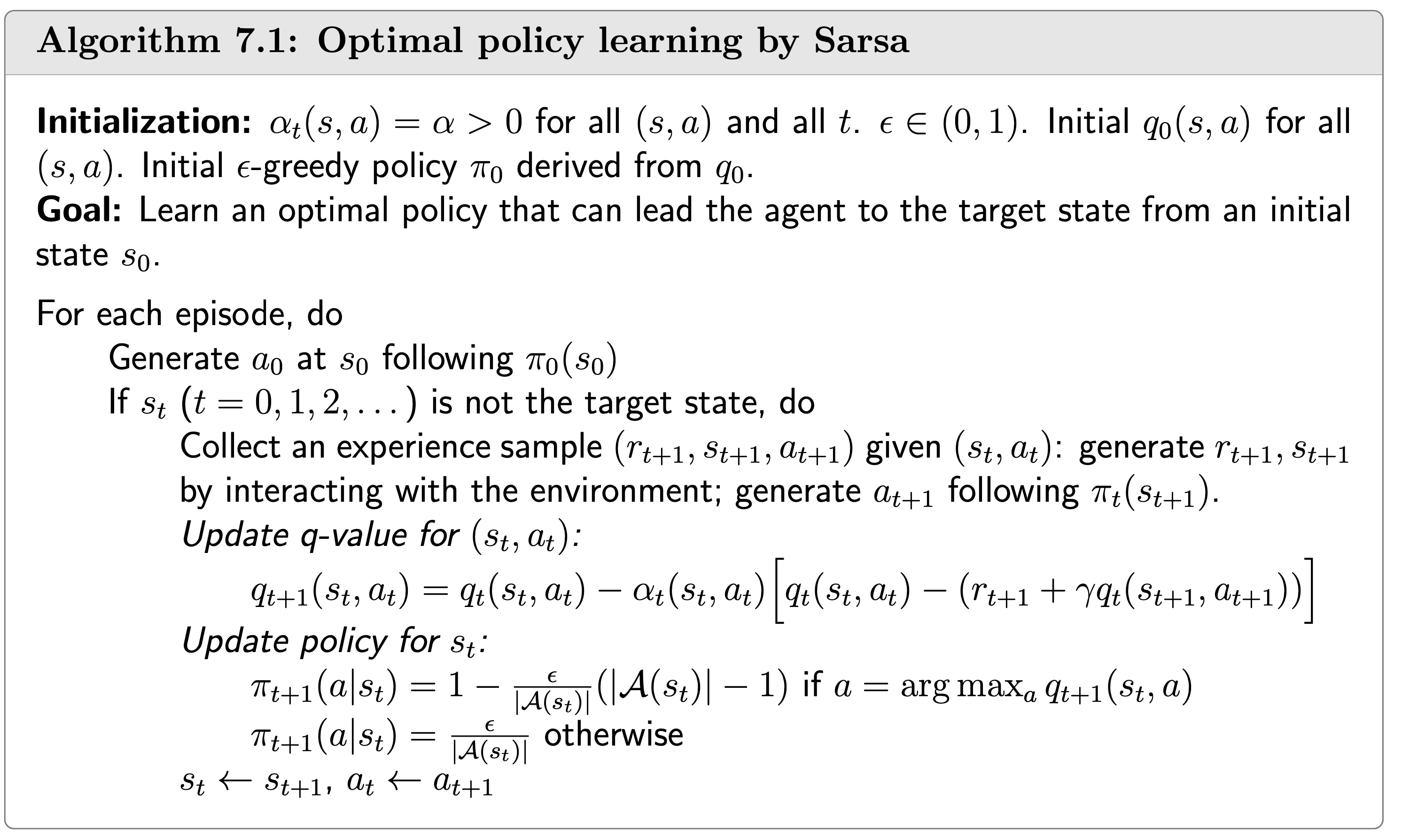
Given the data/experience ${\left\{(s_t,a_t,r_{t+1},s_{t+1},a_{t+1})\right\}}_t$ generated following the given policy $\pi$, the TD learning algorithm (Sarsa) to estimate the action value function of policy $\pi$ is: $$\begin{array}{rl}{q}_{t+1}(s_t,a_t)& =q_t(s_t,a_t)-{\alpha }_t(s_t,a_t)[q_t(s_t,a_t)-[r_{t+1}+\gamma q_t(s_{t+1},a_{t+1})]]\\ q_{t+1}(s,a)& =q_t(s,a),\mathrm{\forall }(s,a)\ne (s_t,a_t)\end{array}$$ where $t=0,1,2,\dots$

• $q_t(s_t,a_t)$ is an estimate of $q_{\pi }(s_t,a_t)$;
• ${\alpha }_t(s_t,a_t)$ is the learning rate depending on $s_t,a_t$.

The name "Sarsa" comes from the abbreviation of state-action-reward-state-action. Each step of the algorithm involves $(s_t,a_t,r_{t+1},s_{t+1},a_{t+1})$.

Convergence of the TD learning algorithm

Theorem (Convergence of TD Learning):

By the TD algorithm, $v_t(s)$ converges with probability 1 to $v_{\pi }(s)$ for all $s\in \mathcal{S}$ as $t\to \mathrm{\infty }$ if $\sum _t{\alpha }_t(s)=\mathrm{\infty }$ and $\sum _t{\alpha }_t^2(s)<\mathrm{\infty }$ for all $s\in \mathcal{S}$.

Remarks: - This theorem says the state value can be found by the TD algorithm for a given a policy $\pi$. - $\sum _t{\alpha }_t(s)=\mathrm{\infty }$ and $\sum _t{\alpha }_t^2(s)<\mathrm{\infty }$ must be valid for all $s\in \mathcal{S}$. At time step $t$, if $s=s_t$ which means that $s$ is visited at time $t$, then ${\alpha }_t(s)>0$; otherwise, ${\alpha }_t(s)=0$ for all the other $s\ne s_t$. That requires every state must be visited an infinite (or sufficiently many) number of times. - The learning rate $\alpha$ is often selected as a small constant. In this case, the condition that $\sum _t{\alpha }_t^2(s)<\mathrm{\infty }$ is invalid anymore. When $\alpha$ is constant, it can still be shown that the algorithm converges in the sense of expectation sense.

For the proof of the theorem, see the book.