Properties of the Fourier Transform
Sources:
- B. P. Lathi & Roger Green. (2018). Chapter 7: Continuous-Time Signal Analysis: The Fourier Transform. Signal Processing and Linear Systems (3nd ed., pp. 701-720). Oxford University Press.
For a quick reference table, see Wikipedia page on the Fourier transform.
Linearity
The Fourier transform is linear; that is, if \[ x_1(t) \Longleftrightarrow X_1(\omega) \quad \text { and } \quad x_2(t) \Longleftrightarrow X_2(\omega) \] then \[ a_1 x_1(t)+a_2 x_2(t) \Longleftrightarrow a_1 X_1(\omega)+a_2 X_2(\omega) \]
The proof is trivial.
conjugation property
The conjugation property states that if \(x(t) \Longleftrightarrow X(\omega)\), then \[ x^*(t) \Longleftrightarrow X^*(-\omega) \]
From this property follows the conjugate symmetry property, also introduced earlier, which states that if \(x(t)\) is real, then \[ X(-\omega)=X^*(\omega) \]
Duality
The duality property states that if \[ x(t) \Longleftrightarrow X(\omega) \] then \[ \begin{equation} \label{eq7_25} X(t) \Longleftrightarrow 2 \pi x(-\omega) \end{equation} \]
Proof:
From the deginition of Fourier transform, we can write \[ x(t)=\frac{1}{2 \pi} \int_{-\infty}^{\infty} X(u) e^{j u t} d u \]
Hence, \[ 2 \pi x(-t)=\int_{-\infty}^{\infty} X(u) e^{-j u t} d u \]
Changing \(t\) to \(\omega\) yields \(\eqref{eq7_25}\)
The scaling property
If \[ x(t) \Longleftrightarrow X(\omega) \] then, for any real constant \(a\), \[ \begin{equation} \label{eq7_26} x(a t) \Longleftrightarrow \frac{1}{|a|} X\left(\frac{\omega}{a}\right) \end{equation} \]
Proof. For a positive real constant \(a\), \[ \mathcal{F}[x(a t)]=\int_{-\infty}^{\infty} x(a t) e^{-j \omega t} d t=\frac{1}{a} \int_{-\infty}^{\infty} x(u) e^{(-j \omega / a) u} d u=\frac{1}{a} X\left(\frac{\omega}{a}\right) \]
Similarly, we can demonstrate that if \(a<0\), \[ x(a t) \Longleftrightarrow \frac{-1}{a} X\left(\frac{\omega}{a}\right) \]
Hence follows \(\eqref{eq7_26}\).
The time-shifting property
If \[ x(t) \Longleftrightarrow X(\omega) \] then \[ x\left(t-t_0\right) \Longleftrightarrow X(\omega) e^{-j \omega t_0} \]
Proof. By definition, \[ \mathcal{F}\left[x\left(t-t_0\right)\right]=\int_{-\infty}^{\infty} x\left(t-t_0\right) e^{-j \omega t} d t \]
Letting \(t-t_0=u\), we have \[ \mathcal{F}\left[x\left(t-t_0\right)\right]=\int_{-\infty}^{\infty} x(u) e^{-j \omega\left(u+t_0\right)} d u=e^{-j \omega t_0} \int_{-\infty}^{\infty} x(u) e^{-j \omega u} d u=X(\omega) e^{-j \omega t_0} \]
This result shows that delaying a signal by \(t_0\) seconds does not change its amplitude spectrum. The phase spectrum, however, is changed by \(-\omega t_0\).
The frequency-shifting property
If \[ x(t) \Longleftrightarrow X(\omega) \] then \[ \color{pink}{x(t) e^{j \omega_0 t} \Longleftrightarrow X\left(\omega-\omega_0\right)} \]
Proof
By definition, \[ \mathcal{F}\left[x(t) e^{j \omega_0 t}\right]=\int_{-\infty}^{\infty} x(t) e^{j \omega_0 t} e^{-j \omega t} d t=\int_{-\infty}^{\infty} x(t) e^{-j\left(\omega-\omega_0\right) t} d t=X\left(\omega-\omega_0\right) \]
According to this property, the multiplication of a signal by a factor \(e^{j \omega_0 t}\) shifts the spectrum of that signal by \(\omega=\omega_0\). Note the duality between the time-shifting and the frequency-shifting properties. Changing \(\omega_0\) to \(-\omega_0\) yields \[ x(t) e^{-j \omega_0 t} \Longleftrightarrow X\left(\omega+\omega_0\right) \]
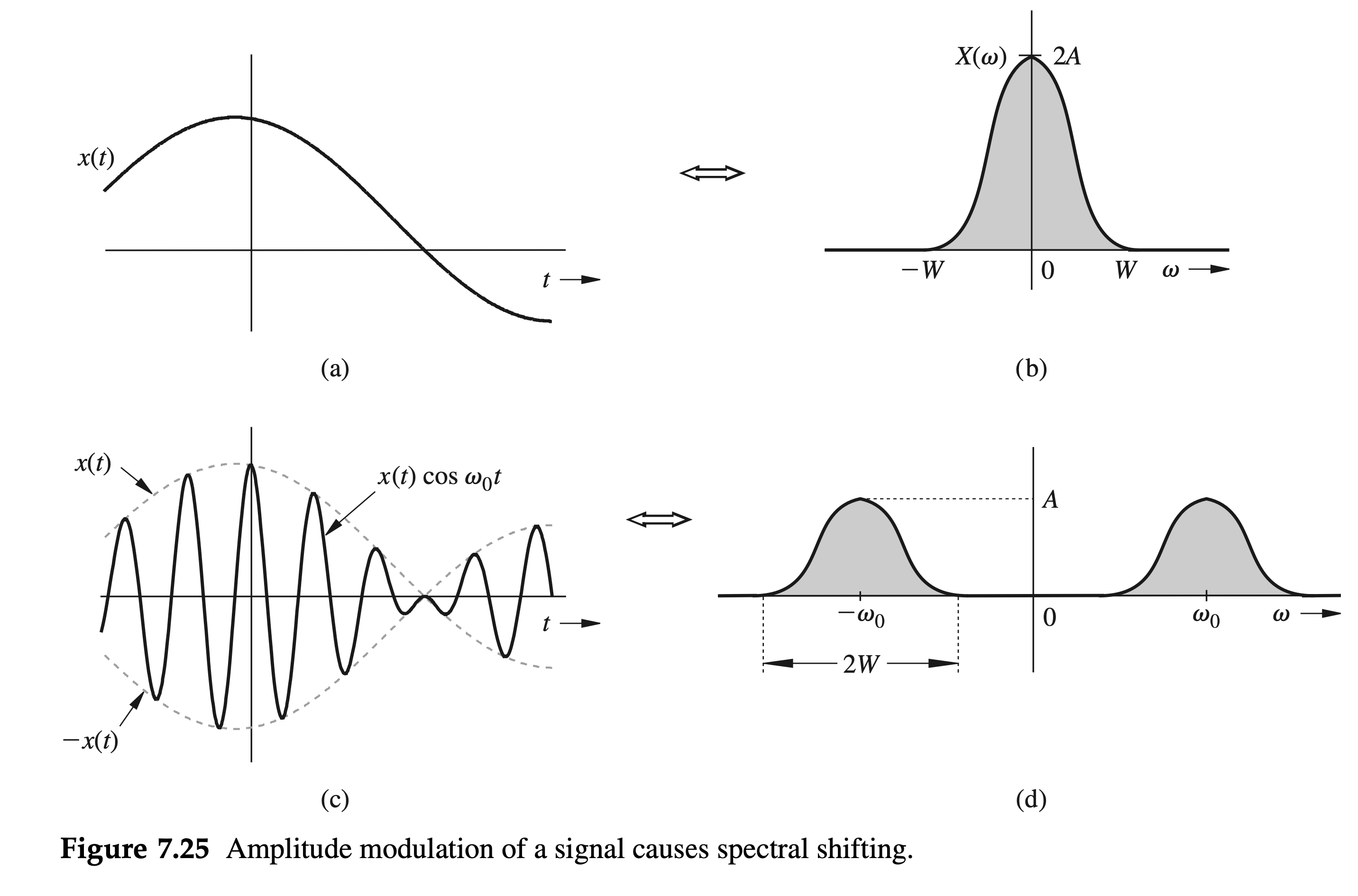
Because \(e^{j \omega_0 t}\) is not a real function that can be generated, frequency shifting in practice is achieved by multiplying \(x(t)\) by a sinusoid. Observe that \[ x(t) \cos \omega_0 t=\frac{1}{2}\left[x(t) e^{j \omega_0 t}+x(t) e^{-j \omega_0 t}\right] \]
we obtain \[ \color{orange}{x(t) \cos \omega_0 t \Longleftrightarrow \frac{1}{2}\left[X\left(\omega-\omega_0\right)+X\left(\omega+\omega_0\right)\right]} \]
This result shows that the multiplication of a signal \(x(t)\) by a sinusoid of frequency \(\omega_0\) shifts the spectrum \(X(\omega)\) by \(\pm \omega_0\), as depicted in Fig. 7.25.