Amplitude Modulation

Sources:

1. B. P. Lathi & Roger Green. (2018). Chapter 7: Continuous-Time Analysis: The Fourier Transform. Signal Processing and Linear Systems (3rd ed., pp. 736-749). Oxford University Press.

Modulation causes a spectral shift in a signal, enhacing long distance transmission. Broadly speaking, there are two classes of modulation: amplitude (linear) modulation and angle (nonlinear) modulation.

In this section, we shall discuss some practical forms of amplitude modulation, including:

1. Double-Sideband, Suppressed-Carrier (DSB-SC) modulation. It is simple and is great for illustrate the idea of amplitude modulation.
2. Amplitude Modulation (AM). It's more efficient than DSB-SC, whereas one more condition must be satisfied. Techinically speaking, all 3 methods in this article belong to amplitude modulation. But it is this specific method which people call amplitude modulation (AM).
3. Single-Sideband, Suppressed-Carrier (DSB-SC) modulation. It is a simpler form of (DSB-SC) modulation where only one sideband is transmitted.

The term Suppressed-Carrier (SC) comes from the fact that, both DSB and SSB signals only contain the modulated signal, excluding the carrrier signal, maing the carrier being "suppressed".

Notatoin

Symbol	Meaning
$m(t)$	The modulating signal or baseband (message) signal.
$B$ Hz	The bandwidth of the signal in hertz. It's the width of the range of positive frequencies for which the amplitue is positive.
$\cos \left({\omega }_{c}t\right)$	The carrier signal used in modulation. The information of a original signal is reflected in either the amplitude or the angle variation of the carrier in the modulated sigal (the modulated sigal contains some transformed form of the carrier), i.e., the carrier "carries" the original signal through modulation.

What is modulation?

Basically, modulation requires doing some computation for an original signal with some carrier signal, which must be a sinusoidal signal, resulting in a modulated signal to be transmitted later. In the modulated signal, the original signal is represented by the either the amplitude or the angle variation of the carrier signal, since the carrier is sinusoidal and a sinusoid is characterized by its amplitude and angle.

When a receiver receives the modulated signal, it extracts the original signal from the variant part. The process is called demodulation.

Take amplitude modulation for example, suppose the original signal, carrier signal and modulated singal are $m(t)$, $\cos \left({\omega }_{c}t\right)$, $m(t)\cos {\omega }_{c}t$ separately, i.e., it's the DSB-SC modulation elaborated later, $m(t)$ is reflected as the amplitude variation of $m(t)\cos {\omega }_{c}t$. This is why DSB-SC modulation belongs to amplitude modulation.

Double-Sideband, Suppressed-Carrier (DSB-SC) modulation

Figure 7.36a

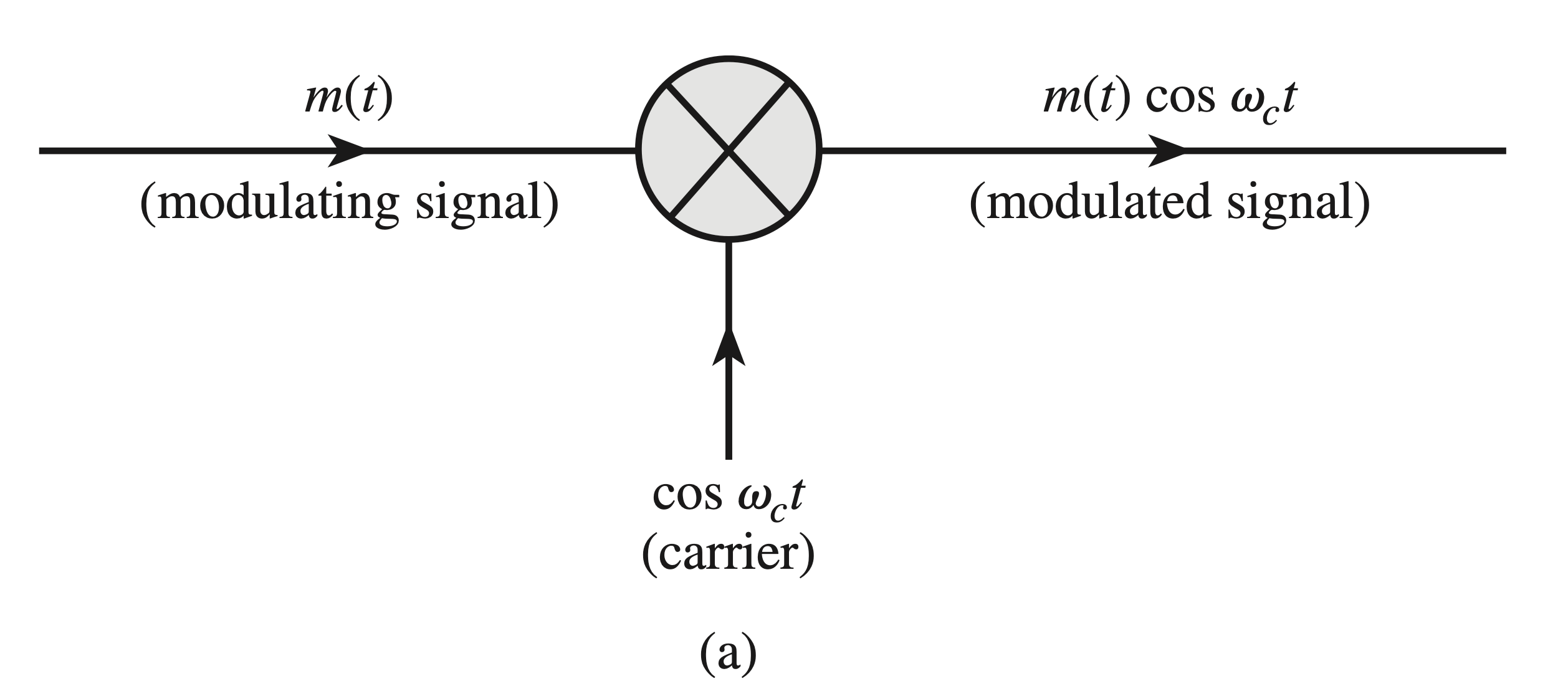
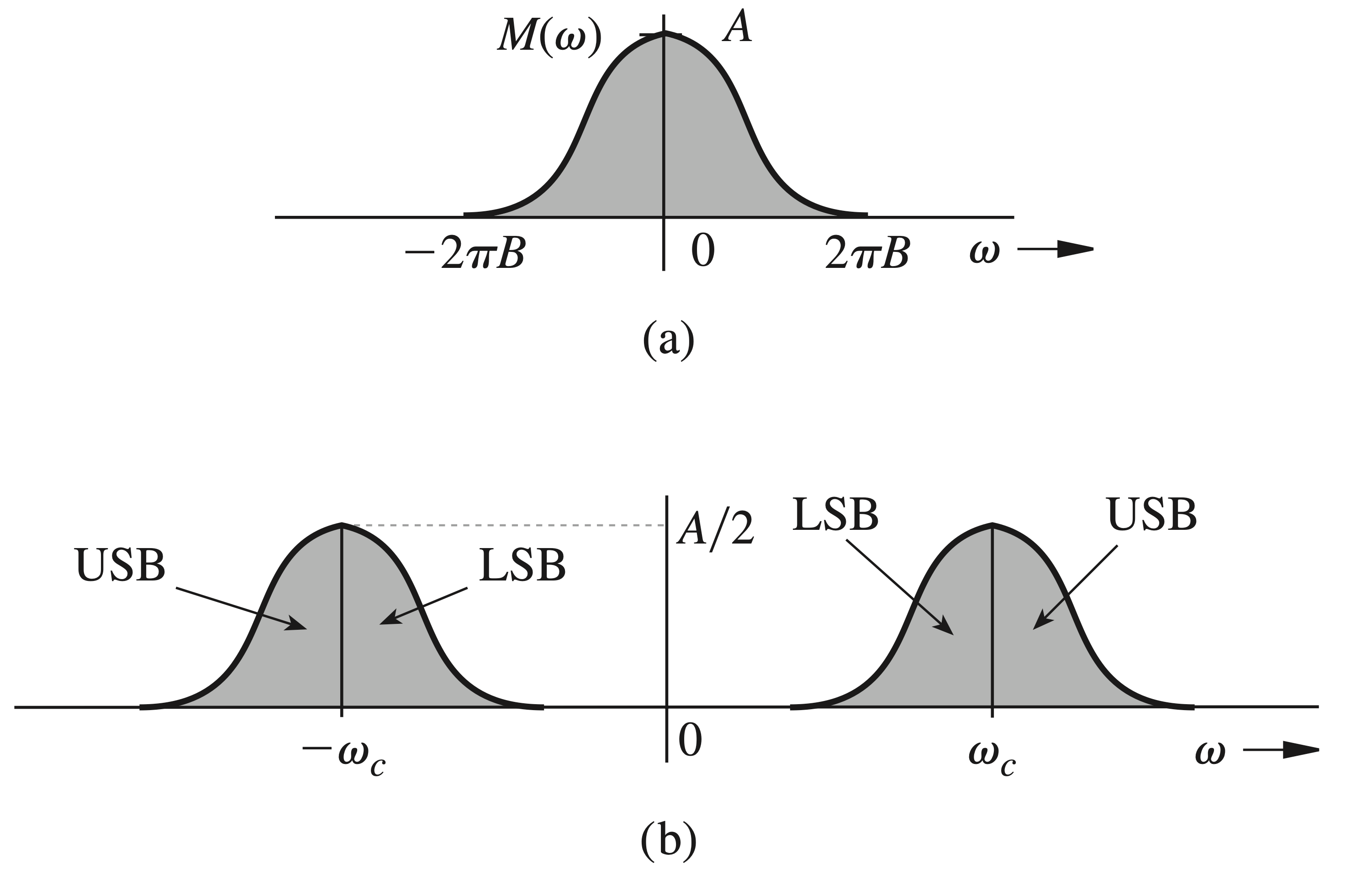
In DSB-SC modulation, given the baseband (message) signal $m(t)$, we multiply it with the carrier $\cos \left({\omega }_{c}t\right)$ in time domain to get the modulated signal $m(t)\cos {\omega }_{c}t$ (Fig. 7.36a).

As was indicated earlier, using the Fourier transform, we have $$x(t)\cos {\omega }_{0}t⟺\frac{1}{2}[X(\omega -{\omega }_0)+X(\omega +{\omega }_0)],$$

where ${\omega }_0$ is a frequency.

Thus, if $$m(t)⟺M(\omega )$$

then $$m(t)\cos {\omega }_{c}t⟺\frac{1}{2}[M(\omega +{\omega }_c)+M(\omega -{\omega }_c)]$$

Thus, the process of modulation shifts the spectrum of the modulating signal to the left and the right by ${\omega }_c$. Note also that if the bandwidth of $m(t)$ is $B$ Hz, then, as indicated in Fig. 7.36c, the bandwidth of the modulated signal is $2B$ Hz.

Figure 7.36bc

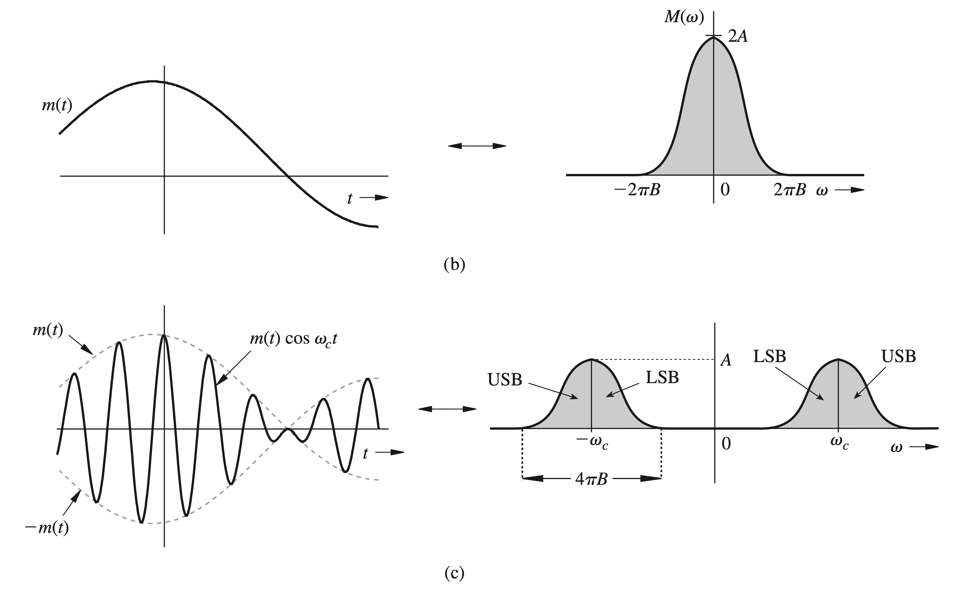
We also observe that the modulated signal spectrum centered at ${\omega }_c$ is composed of two parts:

1. a portion that lies above ${\omega }_c$, known as the upper sideband (USB), and
2. a portion that lies below ${\omega }_c$, known as the lower sideband (LSB).

Similarly, the spectrum centered at $-{\omega }_c$ has upper and lower sidebands. This form of modulation is called double sideband (DSB) modulation for the obvious reason.

Meanwhile, Figure 7.36c shows that, to avoid the overlap of the spectra centered at $\pm {\omega }_c$, $${\omega }_c\ge 2\pi B$$ must be satisfied.

Demodulation of DSB-SC signals

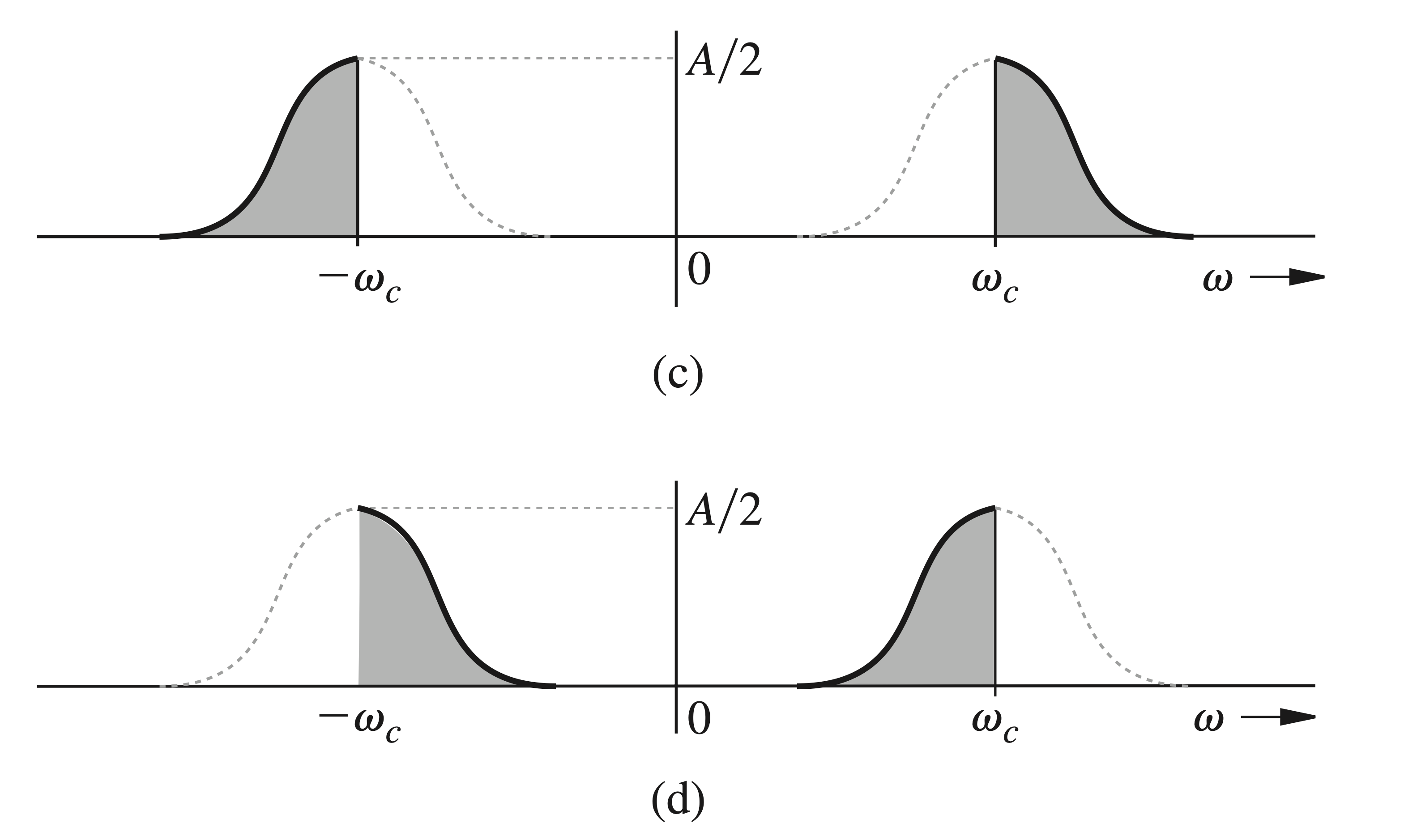
The process of recovering the signal from the modulated signal (retranslating the spectrum to its original position) is referred to as demodulation, or detection. For DSB-SC signals, the demodulation method is called synchronous detection, or coherent detection,

As seen from $$m(t)\cos {\omega }_{c}t⟺\frac{1}{2}[M(\omega +{\omega }_c)+M(\omega -{\omega }_c)],$$ the DSB-SC modulation translates or shifts the frequency spectrum to the left and the right by ${\omega }_c$ (Fig. 7.36c), to recover $m(t)$ from $m(t)\cos {\omega }_{c}t$, we

1. Retranslate the spectrum to its original position. This is done by multiplication of the incoming modulated signal $m(t)\cos {\omega }_{c}t$ by a carrier $\cos {\omega }_{c}t$,
2. Supress the unwanted spectrum at $\pm 2{\omega }_c$ by a lowpass filter.

The process is depicted in Fig. 7.38a.

NOTE:

• After demodulation, we get $(1/2)m(t)$, we then apply amplitude rescaling, which is very simple, to it, getting $m(t)$. Since the amplitude rescaling is very simple, we ommit it in our discussion.
• This demodulation method is called synchronous detection, or coherent detection, since we use a carrier ($\cos {\omega }_{c}t$) of exactly the same frequency (and phase) as the carrier used for modulation. Thus, for demodulation, we need to generate a local carrier at the receiver with the same frequency and phase, i.e., $\cos {\omega }_{c}t$, as the carrier used at the modulator.
  • In reality, a transmitter that may be located hundreds or thousands of miles away. This situation calls for a sophisticated receiver, which could be quite costly. Therefore, in practice we shall use the so-called amplitude modulation (AM) method.

Figure 7.38

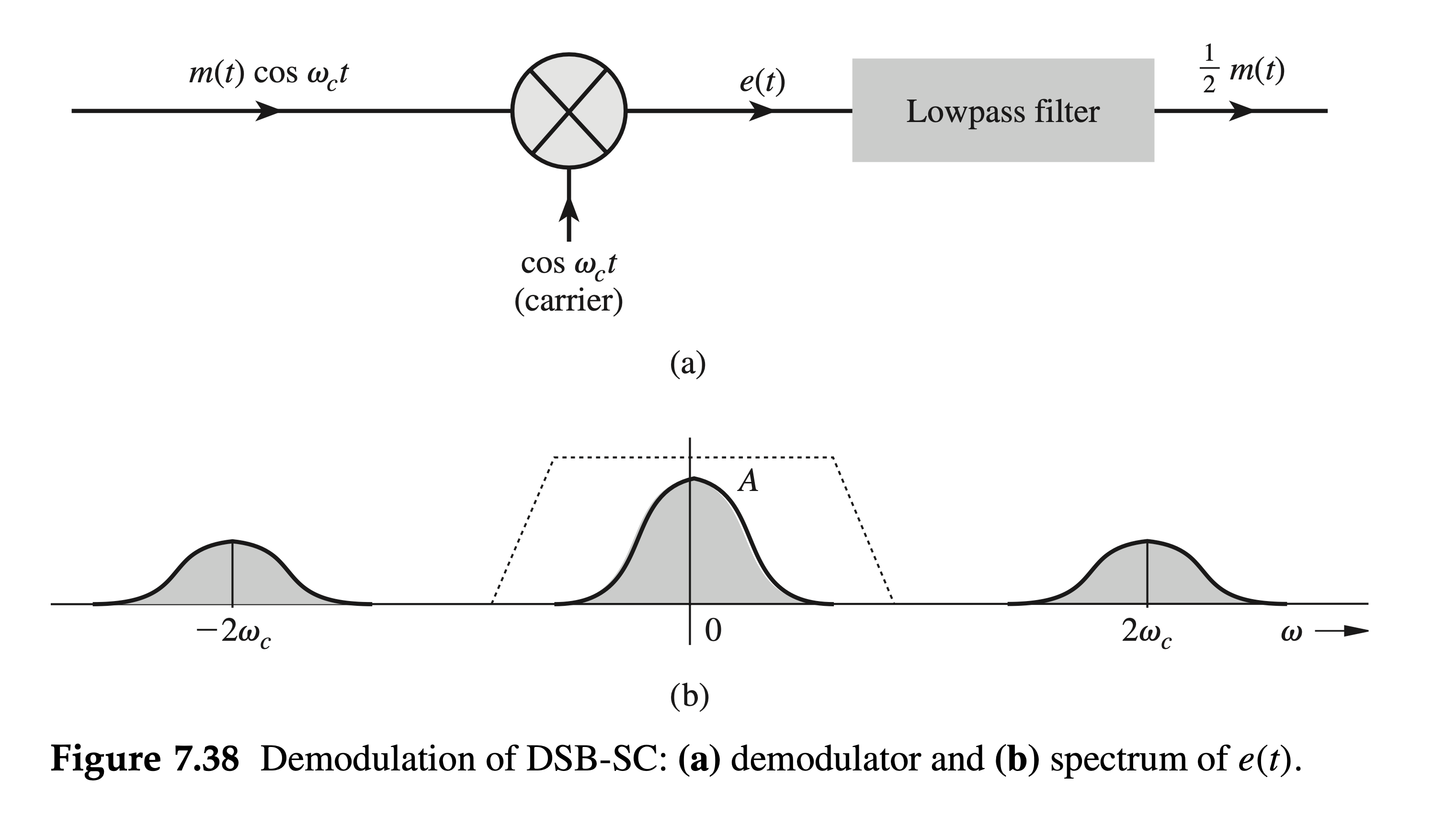
Mathematically speaking, in the first step we are computing the signal $e(t)$ (Fig. 7.38a): $$e(t)=m(t){\cos }^2{\omega }_{c}t=\frac{1}{2}[m(t)+m(t)\cos 2{\omega }_{c}t],$$

whose Fourier transform is $$E(\omega )=\frac{1}{2}M(\omega )+\frac{1}{4}[M(\omega +2{\omega }_c)+M(\omega -2{\omega }_c)].$$

Hence, $e(t)$ consists of two components $(1/2)m(t)$ and $(1/2)m(t)\cos 2{\omega }_{c}t$, with their spectra, as illustrated in Fig. 7.38b.

The spectrum of the second component, being a modulated signal with carrier frequency $2{\omega }_c$, is centered at $\pm 2{\omega }_c$. We filter it out by the lowpass filter in Fig. 7.38a.

After that, we get the desired component $(1/2)M(\omega )$.

Amplitude modulation (AM)

To avoid the overhead of generate a carrier in frequency and phase synchronism with the carrier for a receiver as in DSB-SC modulation, we opt to let the transmitter to transmit a carrier $A\cos {\omega }_{c}t$ (along with the modulated signal $m(t)\cos {\omega }_{c}t]$) so that there is no need to generate a carrier at the receiver.

This is amplitude modulation (AM), in which the transmitted signal ${\phi }_{\mathrm{AM}}(t)$ is given by

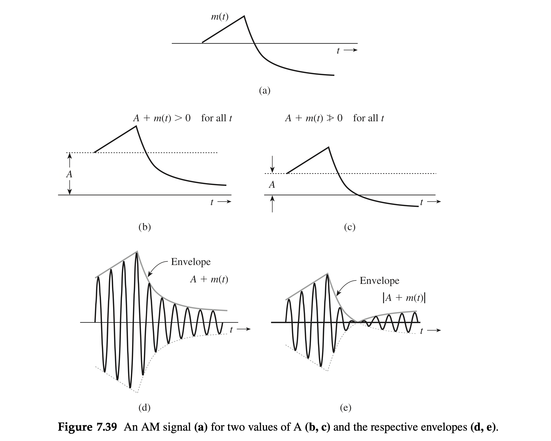
$${\phi }_{\mathrm{AM}}(t)=A\cos {\omega }_{c}t+m(t)\cos {\omega }_{c}t=[A+m(t)]\cos {\omega }_{c}t$$

Recall that the DSB-SC signal is $m(t)\cos {\omega }_{c}t$. Thus, the AM signal is identical to the DSB-SC signal with $A+m(t)$, instead of $m(t)$, as the modulating signal.

To sketch ${\phi }_{\text{AM }}(t)$, we sketch $A+m(t)$ and $-[A+m(t)]$ as the envelopes and fill in between with the sinusoid of the carrier frequency (#TODO). Two cases are considered in Fig. 7.39:

1. In the first case, $A$ is large enough so that $A+m(t)\ge 0$ (is nonnegative) for all values of $t$.
2. In the second case, $A$ is not large enough to satisfy this condition.

In the first case, the envelope (Fig. 7.39d) has the same shape as $m(t)$ (although riding on a dc of magnitude $A$).

In the second case, the envelope shape is not $m(t)$ (#TODO), for some parts get rectified (Fig. 7.39e).

Figure 7.39

Demodulation of AM signals

From the last section, we know that we can detect the desired signal $m(t)$ by detecting the envelope in the first case. In the second case, such a detection is not possible.

The demodulation ethod for AM signals is called envelope detection. We shall see that it's an extremely simple and inexpensive operation since it does not require generation of a local carrier for the demodulation.

But as just noted, the requirement $$A+m(t)\ge 0\text{ for all }t$$ must be satisfied.

If $m_p$ is the peak amplitude (positive or negative) of $m(t)$, then Eq. (7.51) is equivalent to $$A\ge m_p$$

Thus, the minimum carrier amplitude required for the viability of envelope detection is $m_p$. This point is clearly illustrated in Fig. 7.39. We define the modulation index $\mu$ as $$\mu =\frac{m_p}{A}$$ where $A$ is the carrier amplitude. Note that $m_p$ is a constant of the signal $m(t)$. Because $A\ge m_p$ and because there is no upper bound on $A$, it follows that $$0\le \mu \le 1$$

Single-Sideband, Suppressed-Carrier (SSB-SC) modulation

Now consider the baseband spectrum $M(\omega )$ (Fig. 7.42a) and the spectrum of the DSB-SC modulated signal $m(t)\cos {\omega }_{c}t$ (Fig. 7.42b). The DSB spectrum in Fig. 7.42b has two sidebands: the upper and the lower (USB and LSB), both containing complete information on $M(\omega )$ [see Eq. (7.12)].

Clearly, it is redundant to transmit both sidebands. A scheme in which only one sideband is transmitted is known as single-sideband (SSB) transmission, which requires only half the bandwidth of the DSB signal. Thus, we transmit only the upper sidebands (Fig. 7.42c) or only the lower sidebands (Fig. 7.42d).

Figure 7.42cd

Demodulation of SSB-SC signals

An SSB signal can be coherently (synchronously) demodulated. For example, multiplication of a USB signal (Fig. 7.42c) by $2\cos {\omega }_{c}t$ shifts its spectrum to the left and to the right by ${\omega }_c$, yielding the spectrum in Fig. 7.42e.

Lowpass filtering of this signal yields the desired baseband signal. The case is similar with an LSB signal. Hence, demodulation of SSB signals is identical to that of DSB-SC signals, and the synchronous demodulator in Fig. 7.38a can demodulate SSB signals. Note that we are talking of SSB signals without an additional carrier. Hence, they are suppressed-carrier signals (SSB-SC).