DreamerV3 Explanation
Source:
- Papers:
- RSSM
- DreamerV1
- DreamerV2
- DreamerV3
- Blogs:
- EclecticSheep: Dreamer V1
- EclecticSheep: Dreamer V2
- EclecticSheep: Dreamer V3
- EclecticSheep: a2c algorithm
Mastering Diverse Domains through World Models
In my opinion, DreamerV3's success can be attributed to two key factors.
Firstly, it employs a world model based on RSSM, a RNN-like model that incorporates enhanced stochastic elements. This model iteratively generates a latent representation of the real world that is both compressed and temporally coherent, preserving historical information efficiently. This compact and efficient world model significantly contributes to DreamerV3's impressive performance. However, despite its capability to predict future events, DreamerV3 does not exploit this feature, for reasons unknown.
Secondly, DreamerV3 employs various techniques to enhance its adaptability across a range of tasks. These include symlog prediction, free bits strategy, and the unimax categorical distribution
World model inferrence
The world model of DreamerV3 consists of two parts:
- The RSSM, see later.
- The reward and episode continuation (binary) predictors and the decoder.
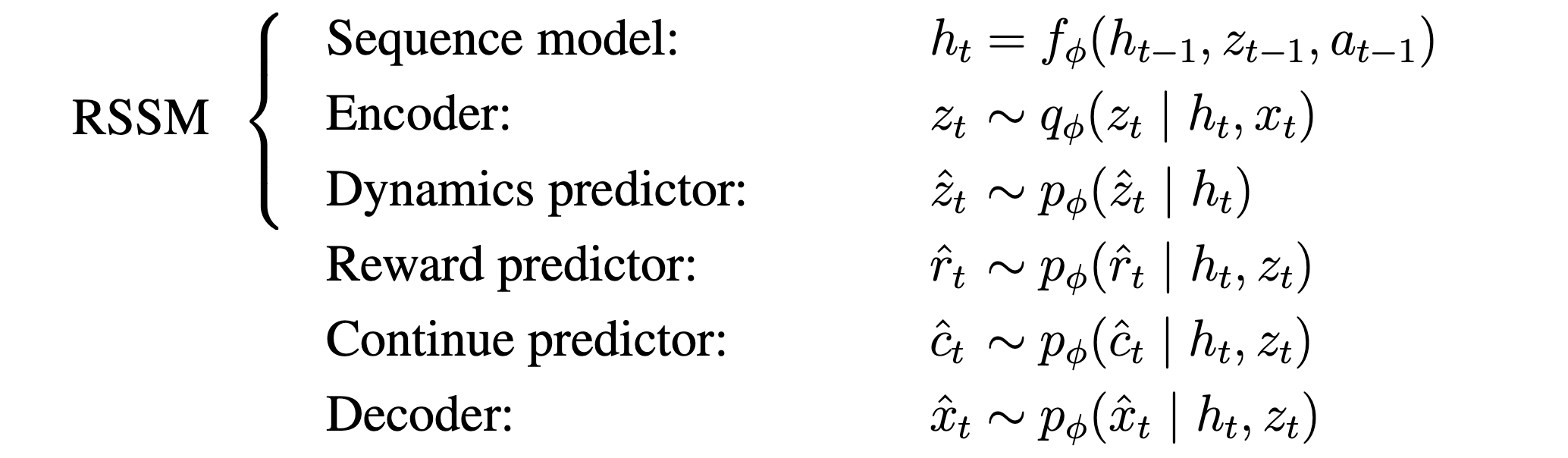
We denote the parameters of the entire world model by \(\phi\).
Note that:
- As the sequence model \(f_{\phi}\) is an RNN, it processes through a deterministic state transition from \(h(t-1)\) to \(h(t)\).
- For simplicity in discussions, the presence of \(h(t)\) can generally be disregarded without altering the outcomes.
- Both the dynamics predictor and the decoder are not utilized during inference.
The inference phase of the world model proceeds as follows
- Encoding Sensory Inputs: The encoder, \(q_\phi\), transforms sensory inputs \(x_t\) and the recurrent state \(h(t)\) (inherent in RNNs) into stochastic categorical representations \(z_t\). This means \(z_t\) is sampled from a stochastic categorical distribution, which is output by both the encoder and the dynamics predictor, not \(z_t\) directly. \[ \text { Encoder: } \quad z_t \sim q_\phi\left(z_t \mid h_t, x_t\right) \]
- State Transition in RNN: The RNN model \(f_\phi\) iteratively carries forward \(h(t)\) and, with the help of the encoder, predicts \(z(t)\) iteratively. \[ \text { Sequence Model: } \quad h_t=f_\phi\left(h_{t-1}, z_{t-1}, a_{t-1}\right) \] Given new \(h(t)\) and \(x(t)\) from the replay buffer during inference, \(q_\phi\) uses them to generate new \(z(t)\) iteratively.
- Model State and Predictions: The concatenation of \(h_t\) and \(z_t\) forms the model state (often called the latent state in literatures), from which rewards \(\hat{r}_t\) and episode continuation flags \(\hat{c}_t\) (binary) are predicted. Similar to \(z_t\), both \(\hat{r}_t\) and \(\hat{c}_t\) are outcomes of stochastic processes, sampled from their respective distributions provided by the reward predictor and crr-tinuation predictor, rather than being output directly.
Question: Given that \(h(t)\) is trivial in RNNs, can I consider the encoder as solely taking \(x(t)\) as input? If \(z(t)\), produced by the encoder, encapsulates the information of \(h(t)\), why not use \(z(t)\) exclusively to predict \(r_t\) and \(c_t\)?
Answer: In the design philosophy of RSSM, \(z_t\) and \(h_t\) represent the stochastic and deterministic states of the real world, respectively. Despite their overlapping information, both are essential for accurate modeling.
RSSM
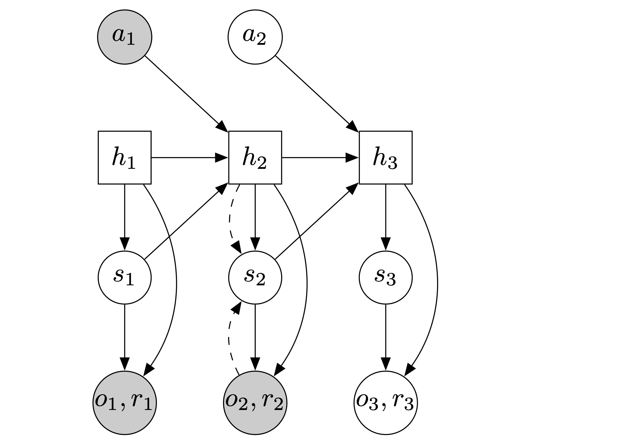
Circles represent stochastic variables and squares deterministic variables. Solid lines denote the generative process and dashed lines the inference model.
Note that the model state, often referred to as the latent state, is formed by concatenating \(h_t\) and \(z_t\). Here, \(h_t\) represents the deterministic component of the world, while \(z_t\) embodies the stochastic aspect. Although \(h_t\) and \(z_t\) may contain overlapping information, their combination is essential for accurately predicting future observations and rewards, as the model state integrates both elements.
World model training
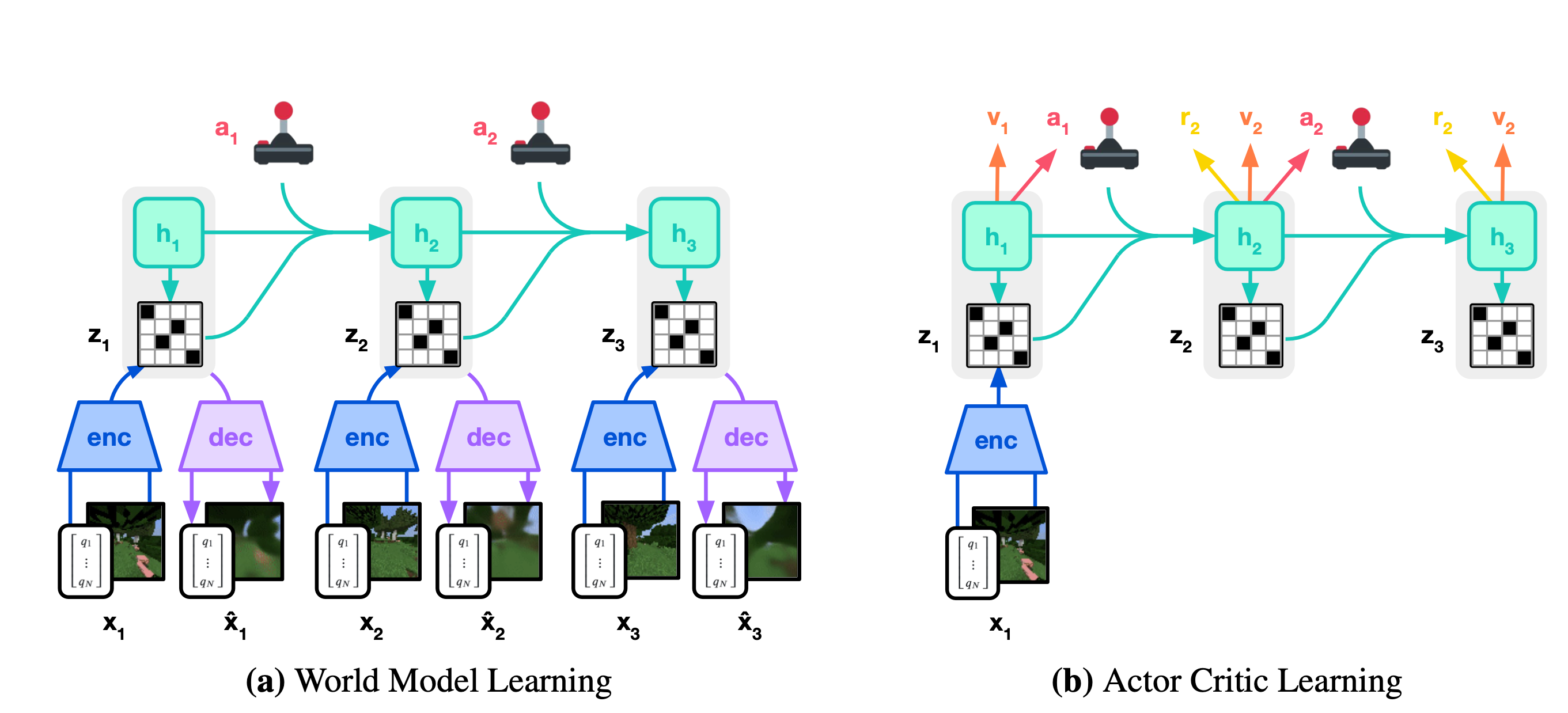
The decoder \(p_\phi\) is trained during the world model traing phase and is not utilized afterwards. Its sole purpose is to facilitate the training of the encoder \(q_\phi\) during this phase. \[ \begin{array}{ll} \text { Encoder: } & z_t \sim q_\phi\left(z_t \mid h_t, x_t\right) \\ \text { Decoder: } & \hat{x}_t \sim p_\phi\left(\hat{x}_t \mid h_t, z_t\right) \end{array} \] The dynamics predictor \(p_\phi\) is also trained during the world model traing phase. Subsequently, it is utilized in the behavior training phase to train the actor-critic.
Although \(p_\phi\) can be leveraged for planning during the inference phase of the RL, the author did not employ it in this manner.
Loss function
Given a sequence batch of inputs \(x_{1: T}\), actions \(a_{1: T}\), rewards \(r_{1: T}\), and continuation flags \(c_{1: T}\), the world model parameters \(\phi\) are optimized end-to-end to minimize the prediction loss \(\mathcal{L}_{\text {pred }}\), the dynamics loss \(\mathcal{L}_{\text {dyn }}\), and the representation loss \(\mathcal{L}_{\text {rep }}\) with corresponding loss weights \(\beta_{\text {pred }}=1, \beta_{\mathrm{dyn}}=1\), and \(\beta_{\mathrm{rep}}=0.1\) :
\[ \mathcal{L}(\phi) \doteq \mathrm{E}_{q_\phi}\left[\sum_{t=1}^T\left(\beta_{\text {pred }} \mathcal{L}_{\text {pred }}(\phi)+\beta_{\mathrm{dyn}} \mathcal{L}_{\text {dyn }}(\phi)+\beta_{\text {rep }} \mathcal{L}_{\text {rep }}(\phi)\right)\right] \] where \[ \begin{aligned} \mathcal{L}_{\text {pred }}(\phi) & \doteq-\ln p_\phi\left(x_t \mid z_t, h_t\right)-\ln p_\phi\left(r_t \mid z_t, h_t\right)-\ln p_\phi\left(c_t \mid z_t, h_t\right) \\ \mathcal{L}_{\text {dyn }}(\phi) & \doteq \max \left(1, \operatorname{KL}\left[\operatorname{sg}\left(q_\phi\left(z_t \mid h_t, x_t\right)\right) \| \quad p_\phi\left(z_t \mid h_t\right)\right]\right) \\ \mathcal{L}_{\text {rep }}(\phi) & \doteq \max \left(1, \operatorname{KL}\left[\quad q_\phi\left(z_t \mid h_t, x_t\right) \| \operatorname{sg}\left(p_\phi\left(z_t \mid h_t\right)\right)\right]\right) \end{aligned} \]
- The prediction loss trains the decoder and reward predictor via the symlog squared loss described later, and the continue predictor via logistic regression.
- The dynamics loss trains the sequence model to predict the next representation by minimizing the KL divergence between the predictor \(p_\phi\left(z_t \mid h_t\right)\) and the next stochastic representation \(q_\phi\left(z_t \mid h_t, x_t\right)\).
- The representation loss, in turn, trains the representations to become more predictable allowing us to use a factorized dynamics predictor for fast sampling during imagination training.
The \(\max (1,.)\) operation is called free bits and will be discussed later.
Explanation of tricks
Symlog function
Differecnt tasks may have different scales of rewards, the reward is a scalar which can be negative, 0, or positive. Some tasks may have reward scale of, say, 0~100; while others may have scales of -1~1.
Meanwile, some tasks have vector observations, and the vectors can have various scales as well. One task may have vector observation whose each element ranges from 0 to 100, whereas the other task may have vector observation whose each element ranges from -10000 to 10.
In this case, for those scalars and vectors, which contains scalars, we must apply some transformations on them to squash them into a more uniform and narrower scople.
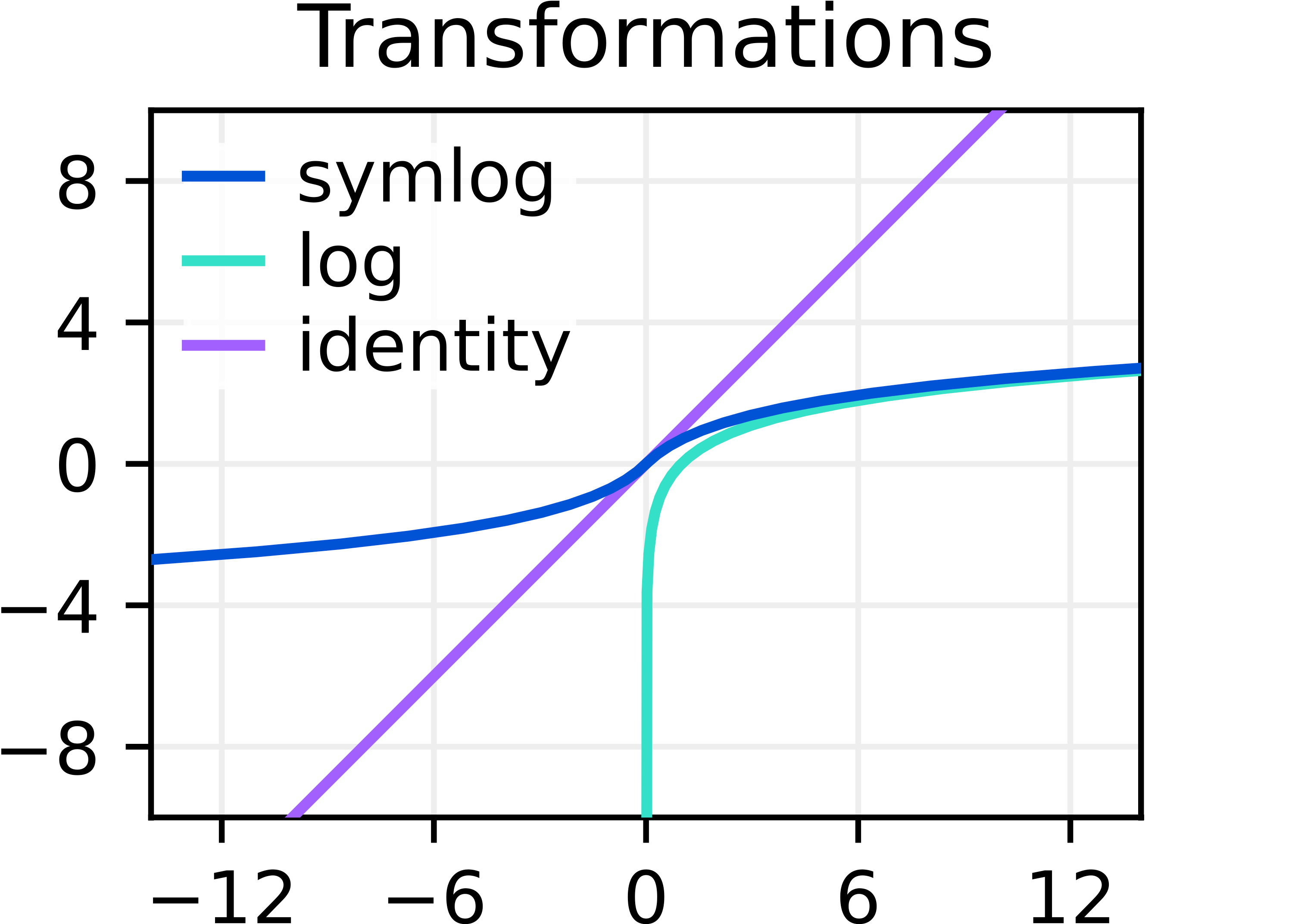
For this reason we introduce symlog() function and its inverse function symexp(), i.e., symexp(symlog(x))=x. \[
\operatorname{symlog}(x) \doteq \operatorname{sign}(x) \ln (|x|+1) \quad \operatorname{symexp}(x) \doteq \operatorname{sign}(x)(\exp (|x|)-1)
\] Say we have a network \(f_{\theta}(x)\) whose output is \(\hat y\), i.e., \[
\hat{y} \doteq (f_\theta(x)),
\] if we transform \(f_{\theta}(x)\) by symlog function, the transformed \(f_{\theta}(x)\) will output \(\operatorname{symlog}(\hat y)\) instead: \[
\operatorname{symlog}{(\hat{y})} \doteq (f_\theta(x)).
\] To read out \(\hat y\) of the network, we apply the inverse function symexp() \[
\hat{y} \doteq \operatorname{symexp}(f_\theta(x)) .
\] DreamerV3 use symlog function to transform the encoder inputs and the decoder targets when the observations are vectors.
For scalars \(\hat r_t\) and \(\hat c_t\), since they are stochastic, i.e., they are sampled from the distrbutions output by the models, we actually read out of them not by symexp(), but by a "modified symexp()"--symexp twohot function.
Symexp twohot function
The rewards and critic neural networks output a softmax distribution over exponentially spaced bins \(b \in B\) and are trained towards twohot encoded targets: \[ \operatorname{twohot}(x)_i \doteq\left\{\begin{array}{ll} \left|b_{k+1}-x\right| /\left|b_{k+1}-b_k\right| & \text { if } i=k \\ \left|b_k-x\right| /\left|b_{k+1}-b_k\right| & \text { if } i=k+1 \\ 0 & \text { else } \end{array} \quad k \doteq \sum_{j=1}^{|B|} \delta\left(b_j<x\right)\right. \]
In this way a nuber \(x\) is represented by a vector of \(K\) numbers, all set to zero except for the two positions corresponding to the two buckets among which is situated \(x\). For instance, if you have 5 buckets which equally divide the range \([0,10]\) (i.e., the 5 buckets are: \([0,2.5,5,7.5,10]\) ) and you have to represent the number \(x=5.5\), then its two hot encoding is the following: \[ \operatorname{twohot}(5.5)=[0,0,0.8,0.2,0] \]
Because 5.5 is closer to bucket 5 than bucket 7.5 .
NOTE: This example is for equally spaced bins, as in old DreamerV3, whereas in the new DreamerV3 we use the exponentially spaced bins.
Free bits
Since the world model of DreamerV3 utilizes a latent representation as its model state, the representation space may collapse, which means the dynamics predicter falls into a trivial solution and predicts sth not containing enough information about the inputs. To tackle this, we use a free bits trick by clipping the dynamics and representation losses below the value of 1 nat ~= 1.44 bits. This disables them from traning the modules while they are already minimized well to focus learning on the prediction loss.
Unimax categorical distribution
The latent representation of the world model, \(z_t\), is sampled from a stochastic categorical distribution output by both the encoder and the dynamics predictor. In practice, however, \(z_t\)'s distribution may approach determinism, leading to spikes in KL losses. To address this, we employ the 'unimix trick,' which involves parameterizing the categorical distributions from the encoder and dynamics predictor as mixtures of 1% uniform and 99% neural network output.