The Bilateral Laplace Transform
Sources:
- B. P. Lathi & Roger Green. (2018). Chapter 4: The Laplace Transform. Signal Processing and Linear Systems (3rd ed., pp. 445-455). Oxford University Press.
As is mentioned in the previous post, we typically use the unilateral Laplace transform instead of the bilateral Laplace transform in that, for a given bilateral Laplace transform \(X(s)\), its inverse Laplace transform is not unique, which is not the case for the unilateral Laplace transform, unless the ROC (Region Of Convergence) is specified.
However, the unilateral Laplace transform can only deal with signal \(x(t)\) starting from \(t=0\). For a signal \(x(t)\) starting from, say \(-\infty\), we can only use the bilateral Laplace transform.
We now show that any bilateral transform can be expressed in terms of two unilateral transforms. It is, therefore, possible to evaluate bilateral transforms from a table of unilateral transforms.
Again, unless otherwise specified, the term Laplace transform refer to the unilateral Laplace transform.
Region of convergence
Consider the function \(x(t)\) appearing in Fig. 4.56a.
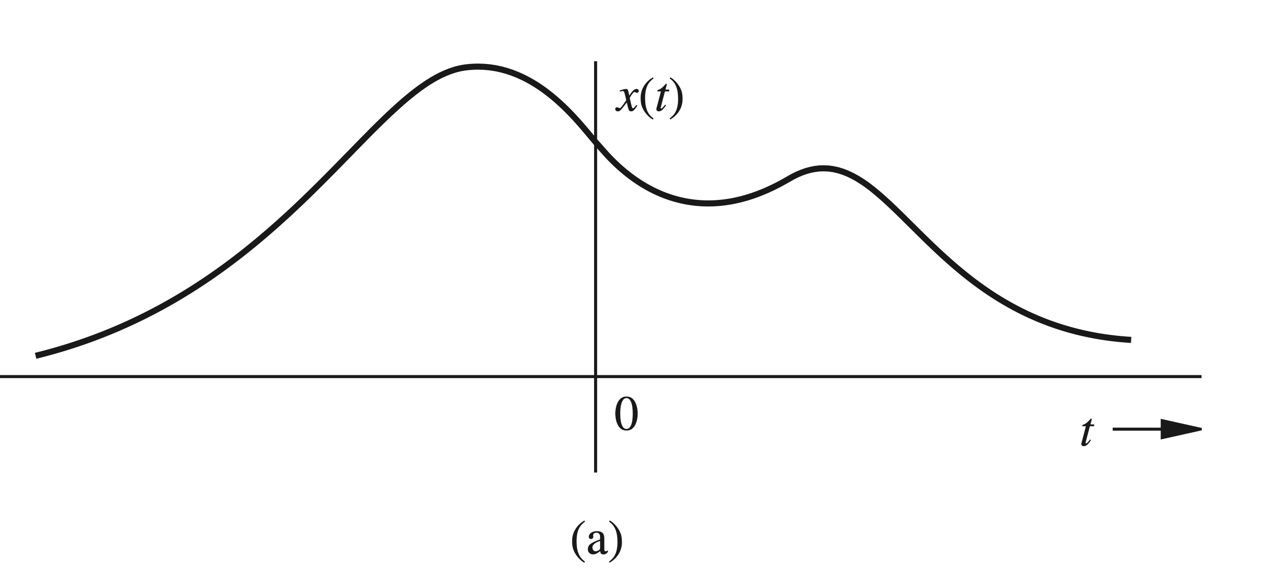
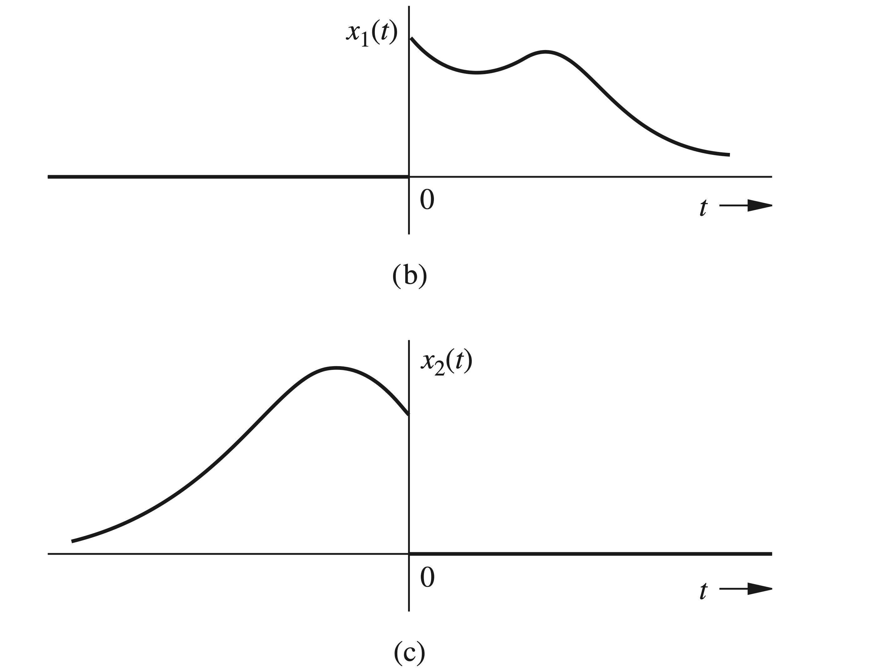
We separate \(x(t)\) into two components, \(x_1(t)\) and \(x_2(t)\), representing the positive time (causal) component and the negative time (anticausal) component of \(x(t)\), respectively (Figs. 4.56b and 4.56c ): \[
x_1(t)=x(t) u(t) \quad \text { and } \quad x_2(t)=x(t) u(-t)
\] 
The bilateral Laplace transform of \(x(t)\) is given by \[ \begin{aligned} X(s) & =\int_{-\infty}^{\infty} x(t) e^{-s t} d t \\ & =\int_{-\infty}^{0^{-}} x_2(t) e^{-s t} d t+\int_{0^{-}}^{\infty} x_1(t) e^{-s t} d t \\ & =X_2(s)+X_1(s) \end{aligned} \] where \(X_1(s)\) is the Laplace transform of the causal component \(x_1(t)\), and \(X_2(s)\) is the Laplace transform of the anticausal component \(x_2(t)\). Consider \(X_2(s)\), given by \[ X_2(s)=\int_{-\infty}^{0^{-}} x_2(t) e^{-s t} d t=\int_{0^{+}}^{\infty} x_2(-t) e^{s t} d t \]
Therefore, \[ X_2(-s)=\int_{0^{+}}^{\infty} x_2(-t) e^{-s t} d t \]
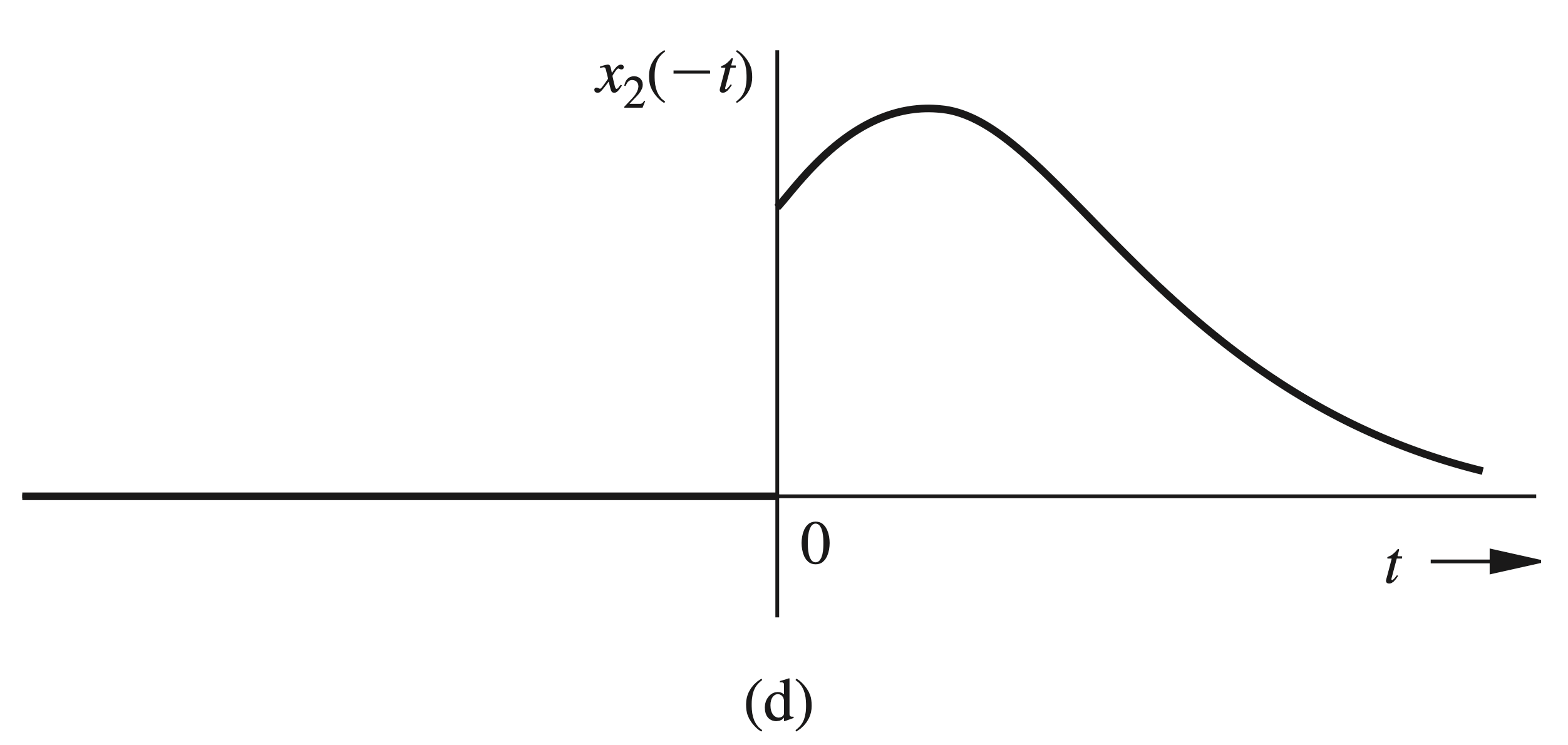
If \(x(t)\) has any impulse or its derivative(s) at the origin, they are included in \(x_1(t)\). Consequently, \(x_2(t)=0\) at the origin; that is, \(x_2(0)=0\). Hence, the lower limit on the integration in the preceding equation can be taken as \(0^{-}\)instead of \(0^{+}\). Therefore, \[ X_2(-s)=\int_{0^{-}}^{\infty} x_2(-t) e^{-s t} d t \]
Because \(x_2(-t)\) is causal (Fig. 4.56d), \(X_2(-s)\) can be found from the unilateral transform table. Changing the sign of \(s\) in \(X_2(-s)\) yields \(X_2(s)\).
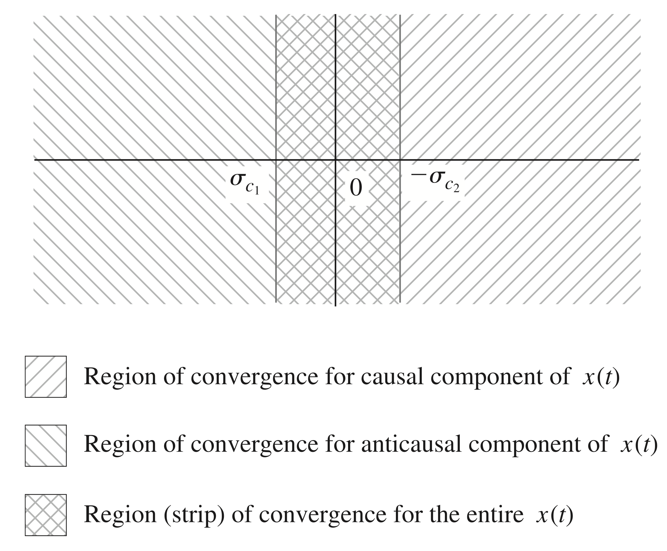
To summarize, the bilateral transform \(X(s)\) in Eq. (4.57) can be computed from the unilateral transforms in two steps: 1. Split \(x(t)\) into its causal and anticausal components, \(x_1(t)\) and \(x_2(t)\), respectively. 2. Since the signals \(x_1(t)\) and \(x_2(-t)\) are both causal, take the (unilateral) Laplace transform of \(x_1(t)\) and add to it the (unilateral) Laplace transform of \(x_2(-t)\), with \(s\) replaced by \(-s\). This procedure gives the (bilateral) Laplace transform of \(x(t)\). Since \(x_1(t)\) and \(x_2(-t)\) are both causal, \(X_1(s)\) and \(X_2(-s)\) are both unilateral Laplace transforms. Let \(\sigma_{c 1}\) and \(\sigma_{c 2}\) be the abscissas of convergence of \(X_1(s)\) and \(X_2(-s)\), respectively. This statement implies that \(X_1(s)\) exists for all \(s\) with \(\operatorname{Re} s>\sigma_{c 1}\), and \(X_2(-s)\) exists for all \(s\) with \(\operatorname{Re} s>\sigma_{c 2}\). Therefore, \(X_2(s)\) exists for all \(s\) with \(\operatorname{Re} s<-\sigma_{c 2} .^{\dagger}\) Therefore, \(X(s)=X_1(s)+X_2(s)\) exists for all \(s\) such that \[ \sigma_{c 1}<\operatorname{Re} s<-\sigma_{c 2} \]
The regions of convergence of \(X_1(s), X_2(s)\), and \(X(s)\) are shown in Fig. 4.57.
Poles and zeros
Because \(X(s)\) is finite for all values of \(s\) lying in the strip of convergence ( \(\sigma_{c 1}<\operatorname{Re} s<-\sigma_{c 2}\) ), poles of \(X(s)\) must lie outside this strip. The poles of \(X(s)\) arising from the causal component \(x_1(t)\) lie to the left of the strip (region) of convergence, and those arising from its anticausal component \(x_2(t)\) lie to its right (see Fig. 4.57). This fact is of crucial importance in finding the inverse bilateral transform.
This result can be generalized to left-sided and right-sided signals. We define a signal \(x(t)\) as a right-sided signal if \(x(t)=0\) for \(t<T_1\) for some finite positive or negative number \(T_1\). A causal signal is always a right-sided signal, but the converse is not necessarily true. A signal is said to left-sided if it is zero for \(t>T_2\) for some finite, positive, or negative number \(T_2\). An anticausal signal is always a left-sided signal, but the converse is not necessarily true. A two-sided signal is of infinite duration on both positive and negative sides of \(t\) and is neither right-sided nor left-sided.
We can show that the conclusions for ROC for causal signals also hold for right-sided signals, and those for anticausal signals hold for left-sided signals. In other words, if \(x(t)\) is causal or
right-sided, the poles of \(X(s)\) lie to the left of the ROC, and if \(x(t)\) is anticausal or left-sided, the poles of \(X(s)\) lie to the right of the ROC.
To prove this generalization, we observe that a right-sided signal can be expressed as \(x(t)+x_f(t)\), where \(x(t)\) is a causal signal and \(x_f(t)\) is some finite-duration signal. The ROC of any finite-duration signal is the entire \(s\)-plane (no finite poles). Hence, the ROC of the right-sided signal \(x(t)+x_f(t)\) is the region common to the ROCs of \(x(t)\) and \(x_f(t)\), which is same as the ROC for \(x(t)\). This proves the generalization for right-sided signals. We can use a similar argument to generalize the result for left-sided signals. Let us find the bilateral Laplace transform of \[ x(t)=e^{b t} u(-t)+e^{a t} u(t) \]
We already know the Laplace transform of the causal component \[ e^{a t} u(t) \Longleftrightarrow \frac{1}{s-a} \quad \operatorname{Re} s>a \]
For the anticausal component, \(x_2(t)=e^{b t} u(-t)\), we have \[ x_2(-t)=e^{-b t} u(t) \Longleftrightarrow \frac{1}{s+b} \quad \operatorname{Re} s>-b \] so that \[ X_2(s)=\frac{1}{-s+b}=\frac{-1}{s-b} \quad \operatorname{Re} s<b \]
Therefore, \[ e^{b t} u(-t) \Longleftrightarrow \frac{-1}{s-b} \quad \operatorname{Re} s<b \] and the Laplace transform of \(x(t)\) in Eq. (4.58) is \[ \begin{aligned} & X(s)=-\frac{1}{s-b}+\frac{1}{s-a} \quad \operatorname{Re} s>a \quad \text { and } \quad \operatorname{Re} s<b \\ & =\frac{a-b}{(s-b)(s-a)} \quad a<\operatorname{Re} s<b \\ & \end{aligned} \]
Figure 4.58 shows \(x(t)\) and the ROC of \(X(s)\) for various values of \(a\) and \(b\). Equation (4.61) indicates that the ROC of \(X(s)\) does not exist if \(a>b\), which is precisely the case in Fig. 4.58f. Observe that the poles of \(X(s)\) are outside (on the edges) of the ROC. The poles of \(X(s)\) because of the anticausal component of \(x(t)\) lie to the right of the ROC, and those due to the causal component of \(x(t)\) lie to its left.
When \(X(s)\) is expressed as a sum of several terms, the ROC for \(X(s)\) is the intersection of (region common to) the ROCs of all the terms. In general, if \(x(t)=\sum_{i=1}^k x_i(t)\), then the ROC for \(X(s)\) is the intersection of the ROCs (region common to all ROCs) for the transforms \(X_1(s), X_2(s)\), \(\ldots, X_k(s)\)
