Practical Lowpass Filters

Sources:

1. B. P. Lathi & Roger Green. (2018). Chapter 4: The Laplace Transform. Signal Processing and Linear Systems (3rd ed., pp. 455-466). Oxford University Press.
2. B. P. Lathi & Roger Green. (2021). Chapter 7: Filter Design by Placement of Poles and Zeros. Signal Processing and Linear Systems (2nd ed., pp. 666-700). Oxford University Press.

Notations

Symbol	Meaning
$G_s$	the maximum stopband gain
$G_p$	the minimum passband gain
${\omega }_c$	the 3 dB cutoff frequency
$\mathcal{H}(s)$	the transfer function of a normalized filter
$H(s)$	the transfer function of a filter
$|H(s)|$	the amplitude response of a filter (or the transfer function)

Practical Filters and Their Specifications

An ideal filter has a passband (unity gain) and a stopband (zero gain) with a sudden transition from the passband to the stopband. There is no transition band. For practical (or realizable) filters, on the other hand, the transition from the passband to the stopband (or vice versa) is gradual and takes place over a finite band of frequencies.

Moreover, for realizable filters, the gain cannot be zero over a finite band (Paley-Wiener condition). As a result, there can be no true stopband for practical filters.

We therefore define a stopband to be a band over which the gain is below some small number $G_s$ (maximum stopband gain), as illustrated in Fig. 7.21.

Similarly, we define a passband to be a band over which the gain is between 1 and some number $G_p(G_p<1)$ ((minimum passband gain)), as shown in Fig. 7.21. We have selected the passband gain of unity for convenience. It could be any constant. Usually, the gains are specified in terms of decibels. This is simply 20 times the log (to base 10) of the gain. Thus, $$\hat{G}(\mathrm{dB})=20{\log }_{10}G$$

A gain of unity is 0 dB and a gain of $\sqrt{2}$ is 3.01 dB, usually approximated by 3 dB.

In a typical design procedure, $G_p$ (minimum passband gain) and $G_s$ (maximum stopband gain) are specified. Figure 7.21 shows the passband, the stopband, and the transition band for typical lowpass, bandpass, highpass, and bandstop filters. In this chapter, we shall discuss design procedures for these four types of filters. Fortunately, highpass, bandpass, and bandstop filters can be obtained from a basic lowpass filter by simple frequency transformations. For example, replacing $s$ with ${\omega }_c/s$ in the lowpass filter transfer function results in a highpass filter. Similarly, other frequency transformations yield the bandpass and bandstop filters. Hence, it is necessary to develop a design procedure only for a basic lowpass filter. Then, by using appropriate transformations, we can design filters of other types. We shall consider here two well-known families of filters: Butterworth and Chebyshev filters.

Butterworth filters

A semicircular wall of poles leads to the Butterworth family of filters, and a semi-elliptical shape leads to the Chebyshev family of filters.

The characteristics of a Chebyshev filter are inferior to those of Butterworth over the passband $(0,{\omega }_c)$, where the characteristics show a rippling effect instead of the maximally flat response of Butterworth. But in the stopband ( $\omega >{\omega }_c$), Chebyshev behavior is superior in the sense that Chebyshev filter gain drops faster than that of the Butterworth.

The amplitude response $|H(j\omega )|$ of an $N$ th-order Butterworth lowpass filter is given by $$\begin{array}{}\text{(1)}& |H(j\omega )|=\frac{1}{\sqrt{1+{\left(\frac{\omega }{{\omega }_c}\right)}^{2N}}}\end{array}$$ Observe that at $\omega =0$, the gain $|H(j0)|$ is unity and at $\omega ={\omega }_c$, the gain $\left|H\left(j{\omega }_c\right)\right|=1/\sqrt{2}$ or -3 $\mathrm{dB}$. The gain drops by a factor $\sqrt{2}$ at $\omega ={\omega }_c$. Because the power is proportional to the amplitude squared, the power ratio (output power to input power) drops by a factor of 2 at $\omega ={\omega }_c$. For this reason, ${\omega }_c$ is called the half-power frequency or the 3 dB cutoff frequency (an amplitude ratio of $\sqrt{2}$ is 3 dB).

Normalized Butterworth Filter

Figure 7.22

In the design procedure, it proves most convenient to consider a normalized filter, denoted as $\mathcal{H}(s)$, whose half-power frequency is 1 rad/s (${\omega }_c=1$). For such a filter, the amplitude characteristic in $\text{(1)}$ reduces to $$\begin{array}{}\text{(2)}& |\mathcal{H}(j\omega )|=\frac{1}{\sqrt{1+{\omega }^{2N}}}\end{array}$$

Once the normalized transfer function $\mathcal{H}(s)$ is obtained, we can obtain the desired transfer function $H(s)$ for any value of ${\omega }_c$ by simple frequency scaling, where we replace $s$ by $s/{\omega }_c$ in $\mathcal{H}(s)$.

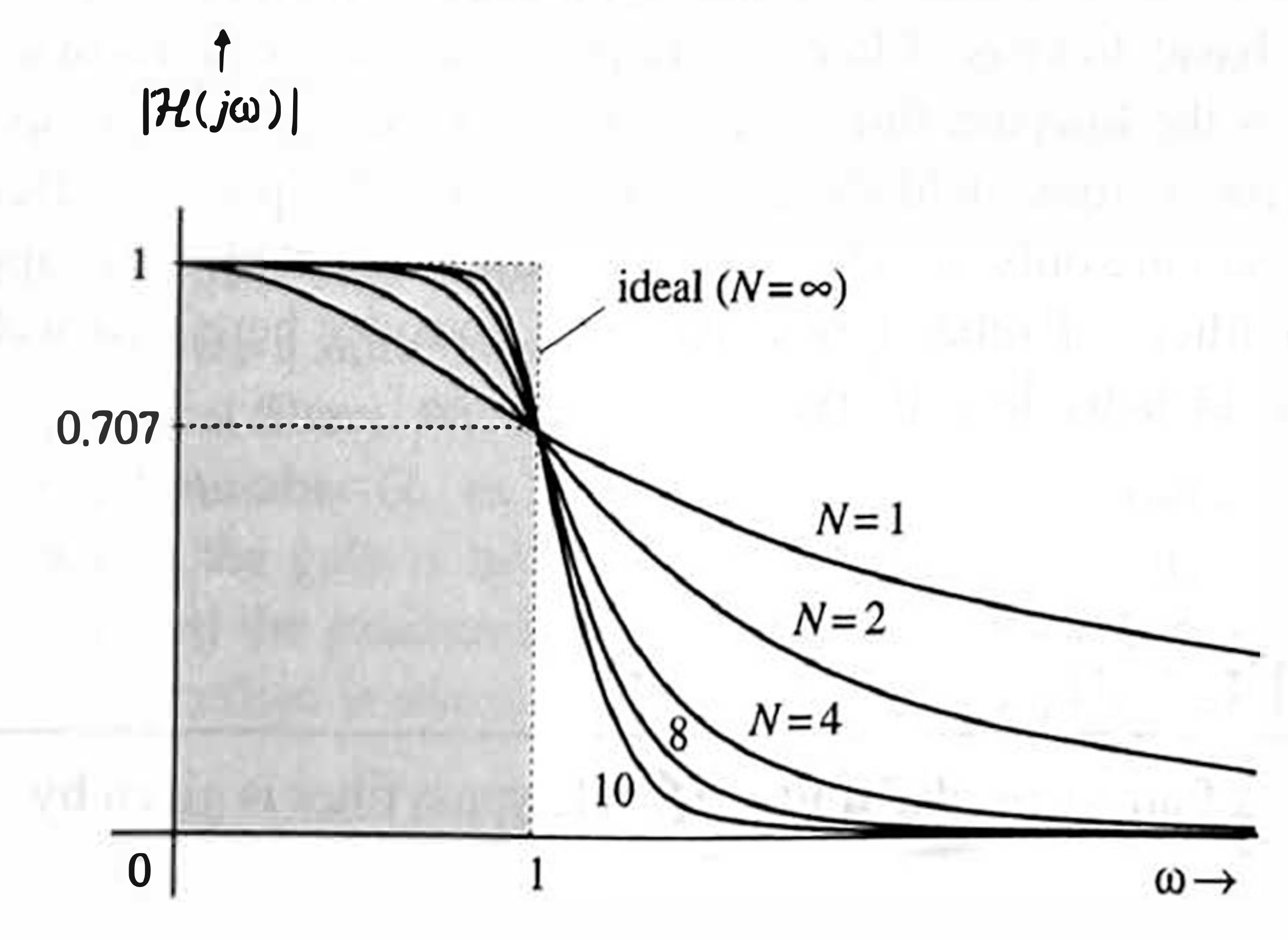
The amplitude responses $|\mathcal{H}(j\omega )|$ of normalized lowpass Butterworth filters are depicted in Fig. 7.22 for various values of $N$. From Fig. 7.22, we observe the following:

1. The Butterworth amplitude response decreases monotonically. Moreover, the first $2\mathrm{N}-1$ derivatives of the amplitude response are zero at $\omega =0$. This characteristic is why Butterworth filters are called maximally flat at $\omega =0$. Observe that a constant characterisic (ideal) is maximally flat for all $\omega <1$. In the Butterworth filter, we try to retain this propenty at least at the origin.
2. The filter gain is 1 (0 dB) at $\omega =0$ and 0.707 (-3 dB) at $\omega =1$ for all $N$. Therefore, the 3 dB (or half power) bandwidth is $1\mathrm{rad}/\mathrm{s}$ for all $N$.
3. For large $N$, the amplitude response approaches the ideal characteristic.

To determine the corresponding transfer function $\mathcal{H}(s)$, recall that $\mathcal{H}(-j\omega )$ is the complex conjugate of $\mathcal{H}(j\omega )$. Therefore, $$\mathcal{H}(j\omega )\mathcal{H}(-j\omega )=|\mathcal{H}(j\omega ){|}^2=\frac{1}{1+{\omega }^{2N}}$$

Substituting $s=j\omega$ in this equation, we obtain $$\mathcal{H}(s)\mathcal{H}(-s)=\frac{1}{1+(s/j{)}^{2N}}$$

The poles of $\mathcal{H}(s)\mathcal{H}(-s)$ occur when $$s^{2N}=-(j{)}^{2N}$$

In this result, we use the fact that $-1=e^{j\pi (2k-1)}$ for integral values of $k$ and $j=e^{j\pi /2}$ to obtain $$s^{2N}=e^{j\pi (2k-1+N)}k\text{ integer }$$

This equation yields the poles of $\mathcal{H}(s)\mathcal{H}(-s)$ as $$\begin{array}{}\text{(3)}& p_k=e^{\frac{j\pi }{2}(2k+N-1)}\end{array}$$

with k=1,2,3, ..., 2N.

Observe that all poles have a unit magnitude; that is, they are located on a unit circle in the $s$ plane separated by angle $\pi /N$, as illustrated in Fig. 7.23 for odd and even $N$.

Figure 7.23

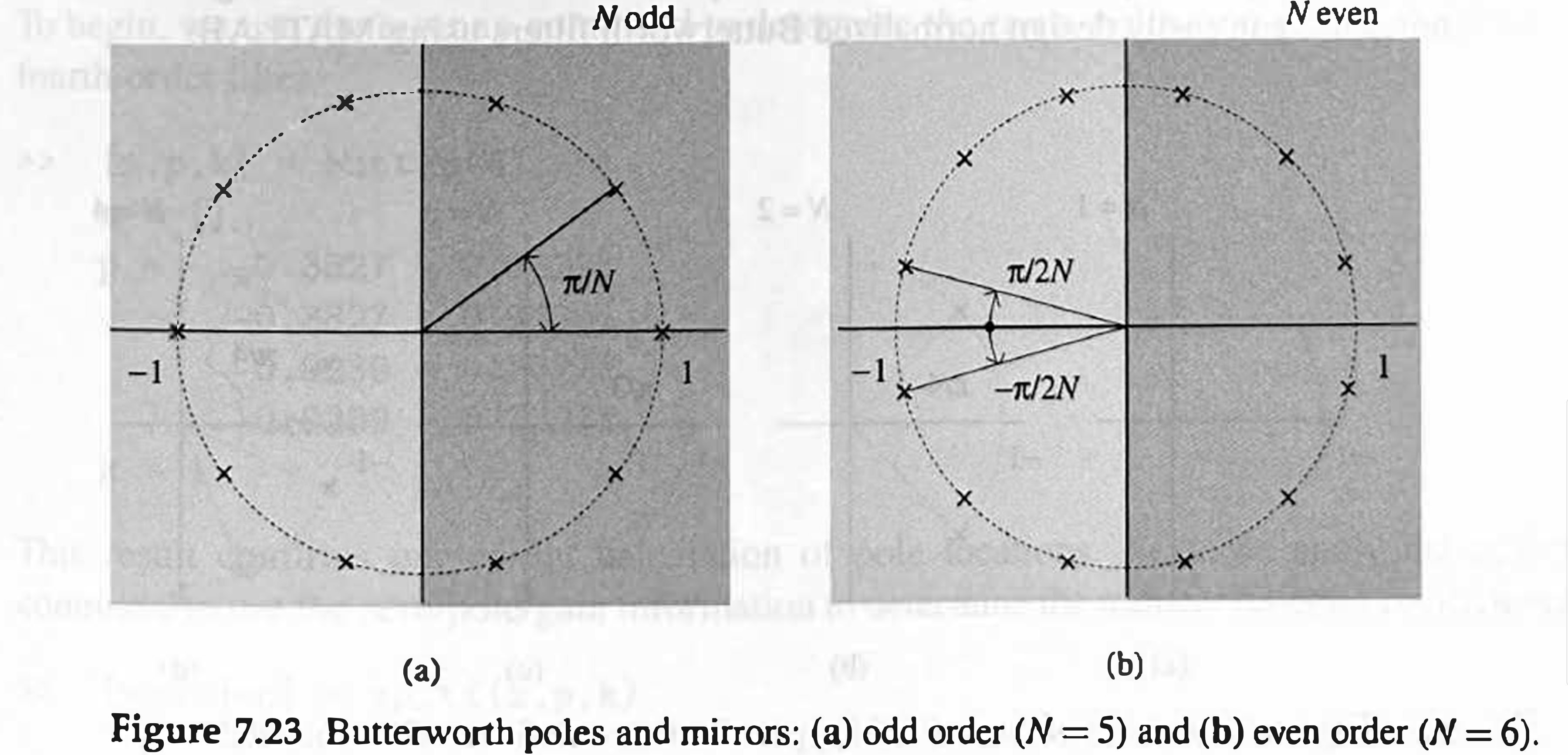
Since $\mathcal{H}(s)$ is stable and causal, its poles must lie in the LHP. The poles of $\mathcal{H}(-s)$ are the mirror images of the poles of $\mathcal{H}(s)$ about the vertical axis. Hence, the poles of $\mathcal{H}(s)$ are those in the LHP and the poles of $\mathcal{H}(-s)$ are those in the RHP in Fig. 7.23.

The poles corresponding to $\mathcal{H}(s)$ are obtained by setting $k=1,2,3,\dots ,N$ in $\text{(3)}$; that is, $$\begin{array}{rl}{p}_k& =e^{\frac{j\pi }{2N}(2k+N-1)}\\ & =\cos \frac{\pi }{2N}(2k+N-1)+j\sin \frac{\pi }{2N}(2k+N-1)k=1,2,3,\dots ,N\end{array}$$ and $\mathcal{H}(s)$ is given by $$\mathcal{H}(s)=\frac{1}{(s-p_1)(s-p_2)\cdots (s-p_N)}$$

For instance, from $$p_k=e^{\frac{j\pi }{2N}(2k+N-1)},$$ we find the poles of $\mathcal{H}(s)$ for $N=4$ occur at angles $$5\pi /8,7\pi /8,9\pi /8,11\pi /8.$$

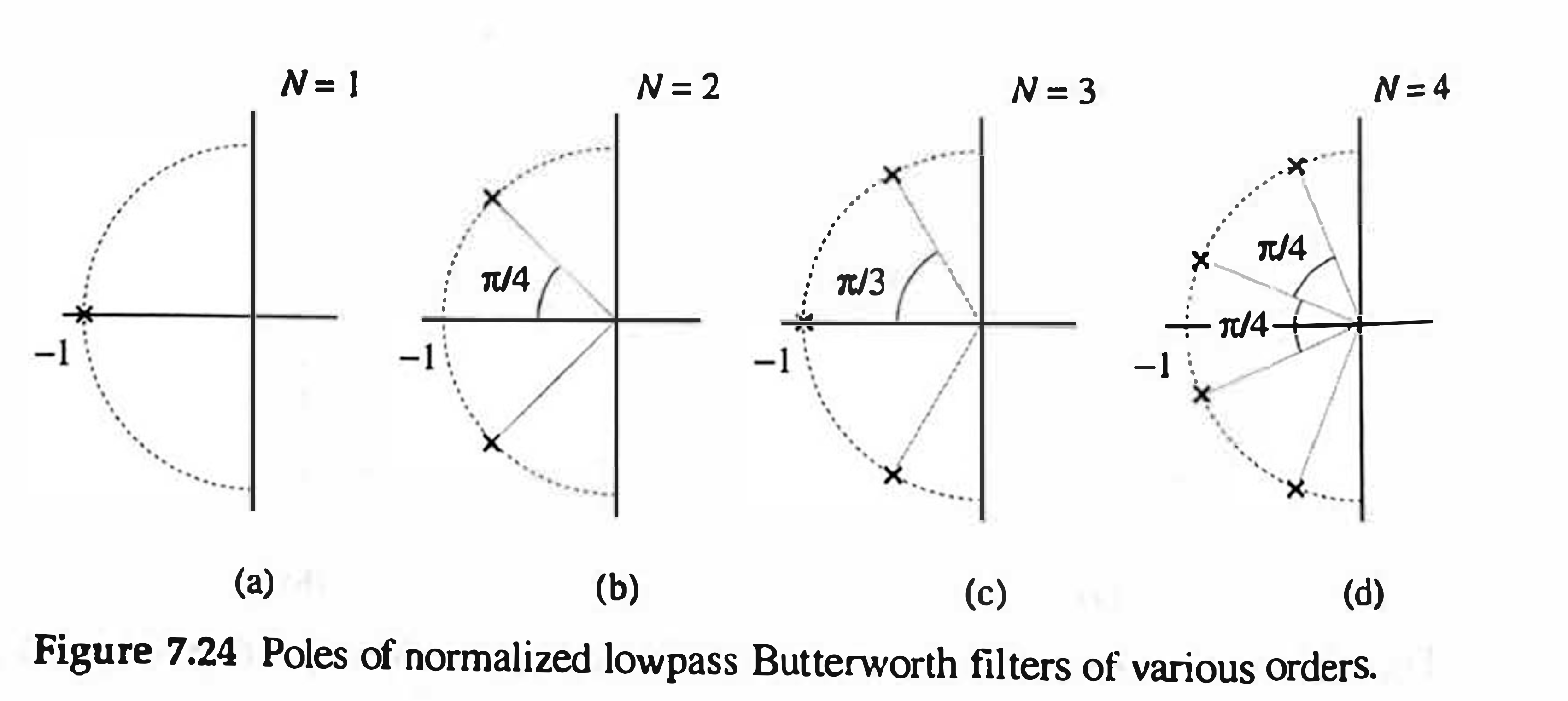
These lie on the unit circle, as shown in Fig. 7.24d, and are given by $-0.3827\pm j0.9239,-0.9239\pm j0.3827$. Hence, $\mathcal{H}(s)$ can be expressed as $$\begin{array}{rl}\mathcal{H}& =\frac{1}{(s+0.38-j0.92)(s+0.38+j0.92)(s+0.92-j0.38)(s+0.92+j0.38)}\\ & =\frac{1}{(s^2+0.7654s+1)(s^2+1.8478s+1)}\\ & =\frac{1}{s^4+2.6131s^3+3.4142s^2+2.6131s+1}\end{array}$$

We can proceed in this way to find $\mathcal{H}(s)$ for any value of $N$. In general, $$\mathcal{H}(s)=\frac{1}{B_N(s)}=\frac{1}{s^N+a_{N-1}{s}^{N-1}+\cdots +a_{1}s+1}$$ where $B_N(s)$ is the Butterworth polynomial of the $N$ th order. Table 7.1 shows the coefficients $a_1$, $a_2,\dots ,a_{N-2},a_{N-1}$ for various values of $N$; Table 7.2 shows $B_N(s)$ in factored form.

Using these tables, we can simply write down our Butterworth filter's transfer function without calculation. For example, using these tables, we read for $N=4$ : $$\begin{array}{rl}\mathcal{H}(s)& =\frac{1}{s^4+2.6131s^3+3.4142s^2+2.6131s+1}\\ & =\frac{1}{(s^2+0.7654s+1)(s^2+1.8478s+1)}\end{array}$$

This result confirms our earlier computations.

Determination of $N$ and ${\omega }_c$

If ${\hat{G}}_x$ is the dB gain of a lowpass Butterworth filter at $\omega ={\omega }_x$, then according to $\text{(1)}$, $${\hat{G}}_x=20{\log }_{10}\left|H\left(j{\omega }_x\right)\right|=-10\log [1+{\left(\frac{{\omega }_x}{{\omega }_c}\right)}^{2N}]$$

Substitution of the specifications in Fig. 7.21a (gains ${\hat{G}}_p$ at ${\omega }_p$ and ${\hat{G}}_s$ at ${\omega }_s$ ) in this equation yields $$\begin{array}{rl}& {\hat{G}}_p=-10\log [1+{\left(\frac{{\omega }_p}{{\omega }_c}\right)}^{2N}]\\ & {\hat{G}}_s=-10\log [1+{\left(\frac{{\omega }_s}{{\omega }_c}\right)}^{2N}]\end{array}$$ or $$\begin{array}{}\text{(4)}& & {\left(\frac{{\omega }_p}{{\omega }_c}\right)}^{2N}={10}^{-{\hat{G}}_p/10}-1\text{(5)}& & {\left(\frac{{\omega }_s}{{\omega }_c}\right)}^{2N}={10}^{-{\hat{G}}_s/10}-1\end{array}$$

Dividing $\text{(4)}$ by $\text{(5)}$, we obtain $${\left(\frac{{\omega }_s}{{\omega }_p}\right)}^{2N}=\left[\frac{{10}^{-{\hat{c}}_s/10}-1}{{10}^{-{\hat{G}}_p/10}-1}\right]$$ and $$N=\frac{\log \left[({10}^{-{\hat{G}}_s/10}-1)/({10}^{-{\hat{G}}_p/10}-1)\right]}{2\log \left({\omega }_s/{\omega }_p\right)}$$

Also from $\text{(4)}$, $${\omega }_c=\frac{{\omega }_p}{{[{10}^{-{\hat{G}}_p/10}-1]}^{1/2N}}$$

Alternatively, from $\text{(5)}$, $${\omega }_c=\frac{{\omega }_s}{{[{10}^{-{\hat{G}}_s/10}-1]}^{1/2N}}$$

Since $N$ is rounded up to an integer value, $\text{(4)}$ and $\text{(5)}$ do not generally return the same value of ${\omega }_c$.

Frequency scaling

Although Tables 7.1 and 7.2 are for normalized Butterworth filters with 3 dB bandwidth ${\omega }_c=1$, the results can be extended to any value of ${\omega }_c$ by simply replacing $s$ by $s/{\omega }_c$. This step implies replacing $\omega$ by $\omega /{\omega }_c$ in Eq. (7.20). For example, a second-order Butterworth filter with ${\omega }_c=100$ can be obtained from Table 7.1 by replacing $s$ by $s/100$ as $$\begin{array}{rl}H(s)& =\frac{1}{{\left(\frac{s}{100}\right)}^2+\sqrt{2}\left(\frac{s}{100}\right)+1}\\ & =\frac{1}{s^2+100\sqrt{2}s+{10}^4}\end{array}$$

The amplitude response $|H(j\omega )|$ of this filter is identical to that of normalized $|\mathcal{H}(j\omega )|$ in $\text{(2)}$, expanded by a factor of 100 along the horizontal ( $\omega$ ) axis (frequency scaling).

Chebyshev Filters

The amplitude response of a normalized Chebyshev lowpass filter is given by $$\begin{array}{}\text{(6)}& |\mathcal{H}(j\omega )|=\frac{1}{\sqrt{1+{ϵ}^2{C}_N^2(\omega )}}\end{array}$$ where $C_N(\omega )$, the $N$ th-order Chebyshev polynomial, is given by $$C_N(\omega )=\cos (N{\cos }^{-1}\omega )\text{ or }{C}_N(\omega )=\cosh (N{\cosh }^{-1}\omega )$$

The first form is most convenient to compute $C_N(\omega )$ for $|\omega |<1$, while the second form is convenient for computing $C_N(\omega )$ for $|\omega |>1$. We can show (see ->here) that $C_N(\omega )$ is also expressible in polynomial form, as shown in Table 7.3 for N=1 to 10.

The normalized Chebyshev lowpass amplitude response $\text{(6)}$ is depicted in Fig. 7.28 for $N=6$ and $N=7$.

Figure 7.28

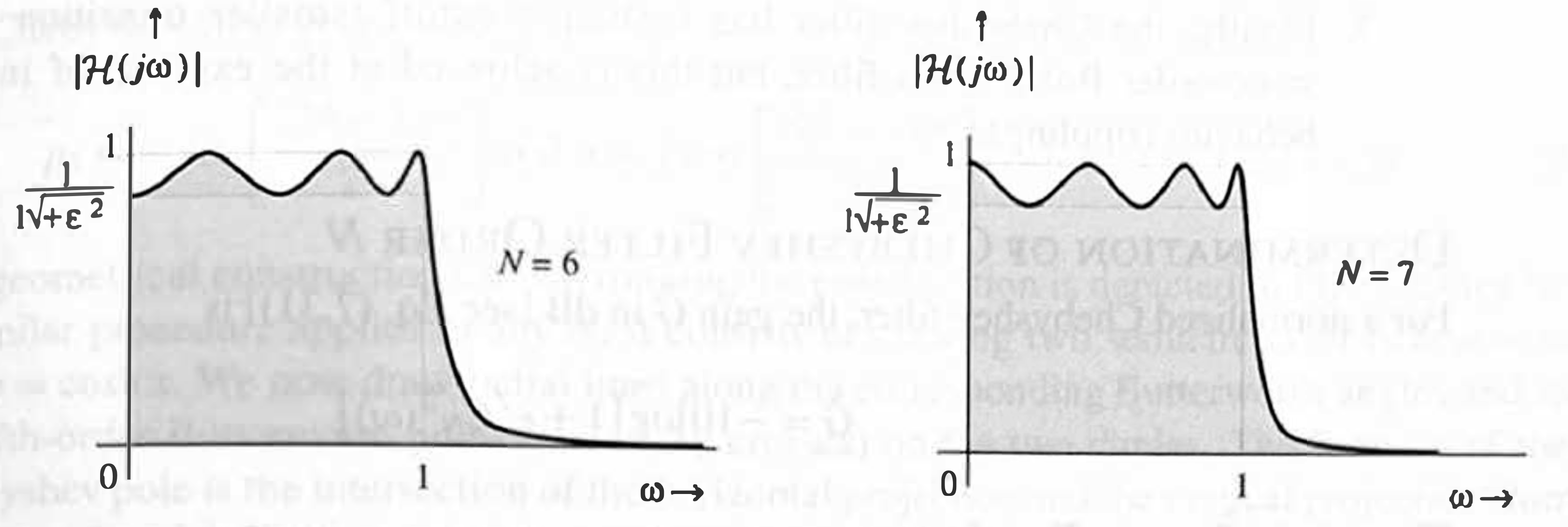
We make the following general observations:

1. The Chebyshev amplitude response has ripples in the passband and is smooth (monotonic) in the stopband. The passband is $0\le \omega \le 1$, and there is a total of $N$ maxima and minims over the passband $0\le \omega \le 1$.
2. From Table 7.3, we observe that $$C_N^2(0)=\{\begin{array}{lc}0& N\text{ odd }\\ 1& N\text{ even }\end{array}$$

Therefore, the dc gain is $$|\mathcal{H}(0)|=\{\begin{array}{cr}1& N\text{ odd }\\ \frac{1}{\sqrt{1+{ϵ}^2}}& N\text{ even }\end{array}$$ 3. The parameter $ϵ$ controls the passband ripple. In the passband, $r$, the ratio of the maximum gain to the minimum gain is $$r=\sqrt{1+{ϵ}^2}$$

This ratio $r$, specified in decibels, is $$\hat{r}=20\log \sqrt{1+{ϵ}^2}=10{\log }_{10}(1+{ϵ}^2)$$ so that $${ϵ}^2={10}^{\hat{r}/10}-1$$

Because all the ripples in the passband are of equal height, Chebyshev polynomials $C_N(\omega )$ are known as equal-ripple functions. 4. Ripple is present only over the passband $0\le \omega \le 1$. At $\omega =1$, the amplitude response is $1/\sqrt{1+{ϵ}^2}=1/r$. For $\omega >1$, the gain decreases monotonically. 5. For Chebyshev filters, the ripple parameter $\hat{r}[\mathrm{dB}]$ takes the place of ${\hat{G}}_p$ (the minimum gain in the passband). For example, $\hat{r}\le 2\mathrm{dB}$ specifies that gain variations of more than $2\mathrm{dB}$ cannot be tolerated in the passband. In a Butterworth filter, ${\hat{G}}_p=-2\mathrm{dB}$ means the same thing. 6. If we reduce the ripple, the passband behavior improves, but it does so at the cost of stopband behavior. As $r$ is decreased ( $ϵ$ is reduced), the gain in the stopband increases, and vice versa. Hence, there is a tradeoff between the allowable passband ripple and the desired attenuation in the stopband. Note that the extreme case $ϵ=0$ yields zero ripple, but the filter now becomes an allpass filter, as seen from $\text{(6)}$ by letting $ϵ=0$.

The Chebyshev polynomial

The Chebyshev polynomial $C_N(x)$ is defined as $$C_N(x)=\cos [N{\cos }^{-1}(x)]=\cosh [N{\cosh }^{-1}(x)]$$

In this form, it is difficult to verify that $C_N(x)$ is a degree-$N$ polynomial in $x$. A recursive form of $C_N(x)$ makes this fact more clear. $$C_N(x)=2x{C}_{N-1}(x)-C_{N-2}(x)$$

With $C_0(x)=1$ and $C_1(x)=x$, the recursive form shows that any $C_N$ is a linear combination of degree- $N$ polynomials and is therefore a degree- $N$ polynomial itself.

Determination of Chebyshev Filter Order $N$

For a normalized Chebyshev filter, the gain $\hat{G}$ in dB (see $\text{(6)}$) is $$\hat{G}=-10\log [1+{ϵ}^2{C}_N^2(\omega )]$$

The gain is ${\hat{G}}_s$ at ${\omega }_s$. Therefore, $${\hat{G}}_s=-10\log [1+{ϵ}^2{C}_N^2\left({\omega }_s\right)]$$ or $${ϵ}^2{C}_N^2\left({\omega }_s\right)={10}^{-{\hat{G}}_s/10}-1$$

The use of $$C_N(\omega )=\cos (N{\cos }^{-1}\omega )\text{ or }{C}_N(\omega )=\cosh (N{\cosh }^{-1}\omega )$$ and $${ϵ}^2={10}^{\hat{r}/10}-1$$ yields $$\cosh [N{\cosh }^{-1}\left({\omega }_s\right)]={\left[\frac{{10}^{-{\hat{\sigma }}_s/10}-1}{{10}^{\hat{r}/10}-1}\right]}^{1/2}$$

Hence, $$N=\frac{1}{{\cosh }^{-1}\left({\omega }_s\right)}{\cosh }^{-1}{\left[\frac{{10}^{-{\hat{G}}_s/10}-1}{{10}^{\hat{r}/10}-1}\right]}^{1/2}$$

Note that these equations are for normalized filters, where ${\omega }_p=1$. For a general case, we replace ${\omega }_s$ with $\frac{{\omega }_s}{{\omega }_p}$ to obtain

#TODO why w_p? $$N=\frac{1}{{\cosh }^{-1}\left({\omega }_s/{\omega }_p\right)}{\cosh }^{-1}{\left[\frac{{10}^{-{\hat{G}}_s/10}-1}{{10}^{\hat{r}/10}-1}\right]}^{1/2}$$

Chebyshev Pole Locations and Normalized Transfer Function

We could follow the procedure of the Butterworth filter to obtain the pole locations of the Chebyshev filter. The procedure is straightforward but tedious and does not yield any sperial insight into our development. Butterworth filter poles lie on a semicircle. We can show tha the poles of an $N$ th-order normalized Chebyshev filter lie on a semiellipse of the major and minor semiaxes $\cosh x$ and $\sinh x$, respectively, where $$x=\frac{1}{N}{\sinh }^{-1}\left(\frac{1}{ϵ}\right)$$ The Chebyshev filter poles are $$p_k=-\sin \left[\frac{(2k-1)\pi }{2N}\right]\sinh x+j\cos \left[\frac{(2k-1)\pi }{2N}\right]\cosh xk=1,2,\cdots ,N$$

The geometrical construction for determining the pole location is depicted in Fig. 7.29 for $N=3$. A similar procedure applies to any $N$; it consists of drawing two semicircles of radii $a=\sinh x$ and $b=\cosh x$. We now draw radial lines along the corresponding Butterworth angles and locate the $N$ th-order Butterworth poles (shown by crosses) on the two circles. The location of the $k$ th Chebyshev pole is the intersection of the horizontal projection and the vertical projection from the corresponding $k$ th Butterworth poles on the outer and inner circles, respectively. The transfer function $\mathcal{H}(s)$ of a normalized $N$ th-order lowpass Chebyshev filter is $$\begin{array}{rl}\mathcal{H}(s)& =\frac{K_N}{(s-p_1)(s-p_2)\cdots (s-p_N)}\\ & =\frac{K_N}{C_N^{\prime }(s)}=\frac{K_N}{s^N+a_{N-1}{s}^{N-1}+\cdots +a_{1}s+a_0}\end{array}$$

The constant $K_N$ is selected following $$|\mathcal{H}(0)|=\{\begin{array}{cr}1& N\text{ odd }\\ \frac{1}{\sqrt{1+{ϵ}^2}}& N\text{ even }\end{array}$$ to provide the proper dc gain:

$$K_N=\{\begin{array}{cc}{a}_0& N\text{ odd }\\ \frac{a_0}{\sqrt{1+{ϵ}^2}}=\frac{a_0}{{10}^{\hat{r}/20}}& N\text{ even }\end{array}$$

Appendix

Table 7.1

Table 7.1 Coefficients of Normalized Butterworth Polynomials

$N$	$a_7$	$a_6$	$a_5$	$a_4$	$a_3$	$a_2$	$a_1$
2							$1.414214$
3						$2.000000$	$2.000000$
4					$2.613126$	$3.414214$	$2.613126$
5				$3.236068$	$5.236068$	$5.236068$	$3.236068$
6			$3.863703$	$7.464102$	$9.141620$	$7.464102$	$3.863703$
7		$4.493959$	$10.097835$	$14.591794$	$14.591794$	$10.097835$	$4.493959$
8	$5.125831$	$13.137071$	$21.846151$	$25.688356$	$21.846151$	$13.137071$	$5.125831$

Table 7.2

Table 7.2 Normalized Butterworth Polynomials in Factored Form

$N$	Normalized Butterworth Polynomials $B_N(s)$, factored form
1	$s+1$
2	$s^2+1.414214s+1$
3	$(s+1)(s^2+s+1)$
4	$(s^2+0.765367s+1)(s^2+1.847759s+1)$
5	$(s+1)(s^2+0.618034s+1)(s^2+1.618034s+1)$
6	$(s^2+0.517638s+1)(s^2+1.414214s+1)(s^2+1.931852s+1)$
7	$(s+1)(s^2+0.445042s+1)(s^2+1.246980s+1)(s^2+1.801938s+1)$
8	$(s^2+0.390181s+1)(s^2+1.111140s+1)(s^2+1.662939s+1)(s^2+1.961571s+1)$

Table 7.3

Table 7.3 Chebyshev polynomials

$N$	$C_N(\omega )$
0	$1$
1	$\omega$
2	$2{\omega }^2-1$
3	$4{\omega }^3-3\omega$
4	$8{\omega }^4-8{\omega }^2+1$
5	$16{\omega }^5-20{\omega }^3+5\omega$
6	$32{\omega }^6-48{\omega }^4+18{\omega }^2-1$
7	$64{\omega }^7-112{\omega }^5+56{\omega }^3-7\omega$
8	$128{\omega }^8-256{\omega }^6+160{\omega }^4-32{\omega }^2+1$
9	$256{\omega }^9-576{\omega }^7+432{\omega }^5-120{\omega }^3+9\omega$
10	$512{\omega }^{10}-1280{\omega }^8+1120{\omega }^6-400{\omega }^4+50{\omega }^2-1$