Frequency Response of An LTIC System

Sources:

1. B. P. Lathi & Roger Green. (2018). Chapter 4: The Laplace Transform. Signal Processing and Linear Systems (3rd ed., pp. 412-419). Oxford University Press.

Response to sinusoidal signals

In the former post I showed that an LTIC system response to an everlasting exponential input $x(t)=e^{st}$ is also an everlasting exponential $H(s)e^{st}$ as long as $s$ is in the region of convergence[^1]. As before, we use an arrow directed from the input to the output to represent an input-output pair: $$\begin{array}{}\text{(1)}& e^{st}⟹H(s)e^{st}\end{array}$$

Setting $s=j\omega$ in this relationship yields $$\begin{array}{}\text{(2)}& e^{j\omega t}⟹H(j\omega )e^{j\omega t}\end{array}$$

Noting that $\cos \omega t$ is the real part of $e^{j\omega t}$, so we have $$\begin{array}{}\text{(3)}& \cos \omega t⟹\mathrm{Re}[H(j\omega )e^{j\omega t}]\end{array}$$

where $[.]$ means "the real part of".

We can express $H(j\omega )$ in the polar form as $$H(j\omega )=|H(j\omega )|e^{j\mathrm{\angle }H(j\omega )}$$

With this result, $\text{(3)}$ becomes $$\cos \omega t⟹|H(j\omega )|\cos [\omega t+\mathrm{\angle }H(j\omega )]$$

In other words, the system response $y(t)$ to a sinusoidal input $\cos \omega t$ is given by $$y(t)=|H(j\omega )|\cos [\omega t+\mathrm{\angle }H(j\omega )]$$

Using a similar argument, we can show that the system response to a sinusoid $\cos (\omega t+\theta )$ is $$\begin{array}{rl}& y(t)=\\ \text{(4)}& & |H(j\omega )|\cos [\omega t+\theta +\mathrm{\angle }H(j\omega )]\end{array}$$ Equation $\text{(4)}$ shows that for a sinusoidal input of radian frequency $\omega$, the system response is also a sinusoid of the same frequency $\omega$. The amplitude of the output sinusoid is $|H(j\omega )|$ times the input amplitude, and the phase of the output sinusoid is shifted by $\mathrm{\angle }H(j\omega )$ with respect to the input phase.

Sometimes we call $|H(j\omega )|$ the amplitude response and call $\mathrm{\angle }H(j\omega )$ the phase response.

Example

Find the frequency response (amplitude and phase responses) of a system whose transfer function is $$H(s)=\frac{s+0.1}{s+5}$$

Also, find the system response $y(t)$ if the input $x(t)$ is (a) $\cos 2t$ (b) $\cos (10t-{50}^{\circ })$

---

In this case, $$H(j\omega )=\frac{j\omega +0.1}{j\omega +5}$$

Therefore, $$|H(j\omega )|=\frac{\sqrt{{\omega }^2+0.01}}{\sqrt{{\omega }^2+25}}\text{ and }\mathrm{\angle }H(j\omega )={\tan }^{-1}\left(\frac{\omega }{0.1}\right)-{\tan }^{-1}\left(\frac{\omega }{5}\right)$$

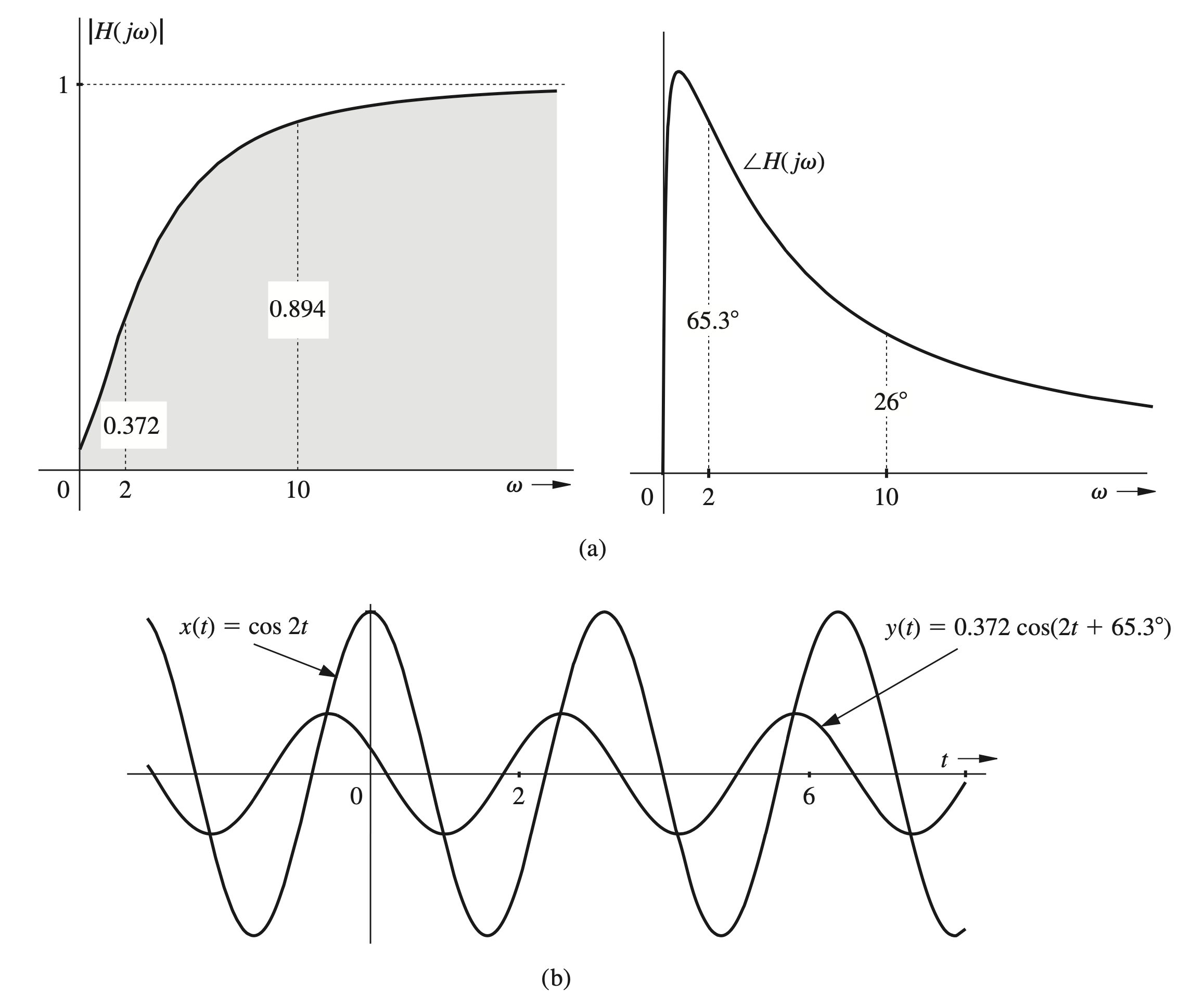
Both the amplitude and the phase response are depicted in Fig. 4.38a as functions of $\omega$. These plots furnish the complete information about the frequency response of the system to sinusoidal inputs.

Figure 4.38

(a)

For the input $x(t)=\cos 2t$, we have $\omega =2$, substitute it into previous equations and get $$\begin{array}{rl}& |H(j2)|=\frac{\sqrt{(2{)}^2+0.01}}{\sqrt{(2{)}^2+25}}=0.372\\ & \mathrm{\angle }H(j2)={\tan }^{-1}\left(\frac{2}{0.1}\right)-{\tan }^{-1}\left(\frac{2}{5}\right)={87.1}^{\circ }-{21.8}^{\circ }={65.3}^{\circ }\end{array}$$ We also could have read these values directly from the frequency response plots in Fig. 4.38a corresponding to $\omega =2$. This result means that for a sinusoidal input with frequency $\omega =2$, the amplitude gain of the system is 0.372 , and the phase shift is ${65.3}^{\circ }$. In other words, the output amplitude is 0.372 times the input amplitude, and the phase of the output is shifted with respect to that of the input by ${65.3}^{\circ }$. Therefore, the system response to the input $\cos 2t$ is $$y(t)=0.372\cos (2t+{65.3}^{\circ })$$

The input $\cos 2t$ and the corresponding system response $0.372\cos (2t+{65.3}^{\circ })$ are illustrated in Fig. 4.38b. ## (b)

For the input $\cos (10t-{50}^{\circ })$, instead of computing the values $|H(j\omega )|$ and $\mathrm{\angle }H(j\omega )$ as in part (a), we shall read them directly from the frequency response plots in Fig. 4.38a corresponding to $\omega =10$. These are $$|H(j10)|=0.894\text{ and }\mathrm{\angle }H(j10)={26}^{\circ }$$

Therefore, for a sinusoidal input of frequency $\omega =10$, the output sinusoid amplitude is 0.894 times the input amplitude, and the output sinusoid is shifted with respect to the input sinusoid by ${26}^{\circ }$. Therefore, the system response $y(t)$ to an input $\cos (10t-{50}^{\circ })$ is $$y(t)=0.894\cos (10t-{50}^{\circ }+{26}^{\circ })=0.894\cos (10t-{24}^{\circ })$$

If the input were $\sin (10t-{50}^{\circ })$, the response would be $0.894\sin (10t-{50}^{\circ }+{26}^{\circ })=$ $0.894\sin (10t-{24}^{\circ })$.

The frequency response plots in Fig. 4.38a show that the system has highpass filtering characteristics; it responds well to sinusoids of higher frequencies ( $\omega$ well above 5), and suppresses sinusoids of lower frequencies ( $\omega$ well below 5 ).

Example: Frequency Responses of Delay, Differentiator, and Integrator Systems

Find and sketch the frequency responses (magnitude and phase) for (a) an ideal delay of $T$ seconds, (b) an ideal differentiator, and (c) an ideal integrator.

Figure 4.39

(a) Ideal delay

The transfer function of an ideal delay is (see -->here) $$H(s)=e^{-sT}$$

Therefore, $$H(j\omega )=e^{-j\omega T}$$

Consequently, $$|H(j\omega )|=1\text{ and }\mathrm{\angle }H(j\omega )=-\omega T$$

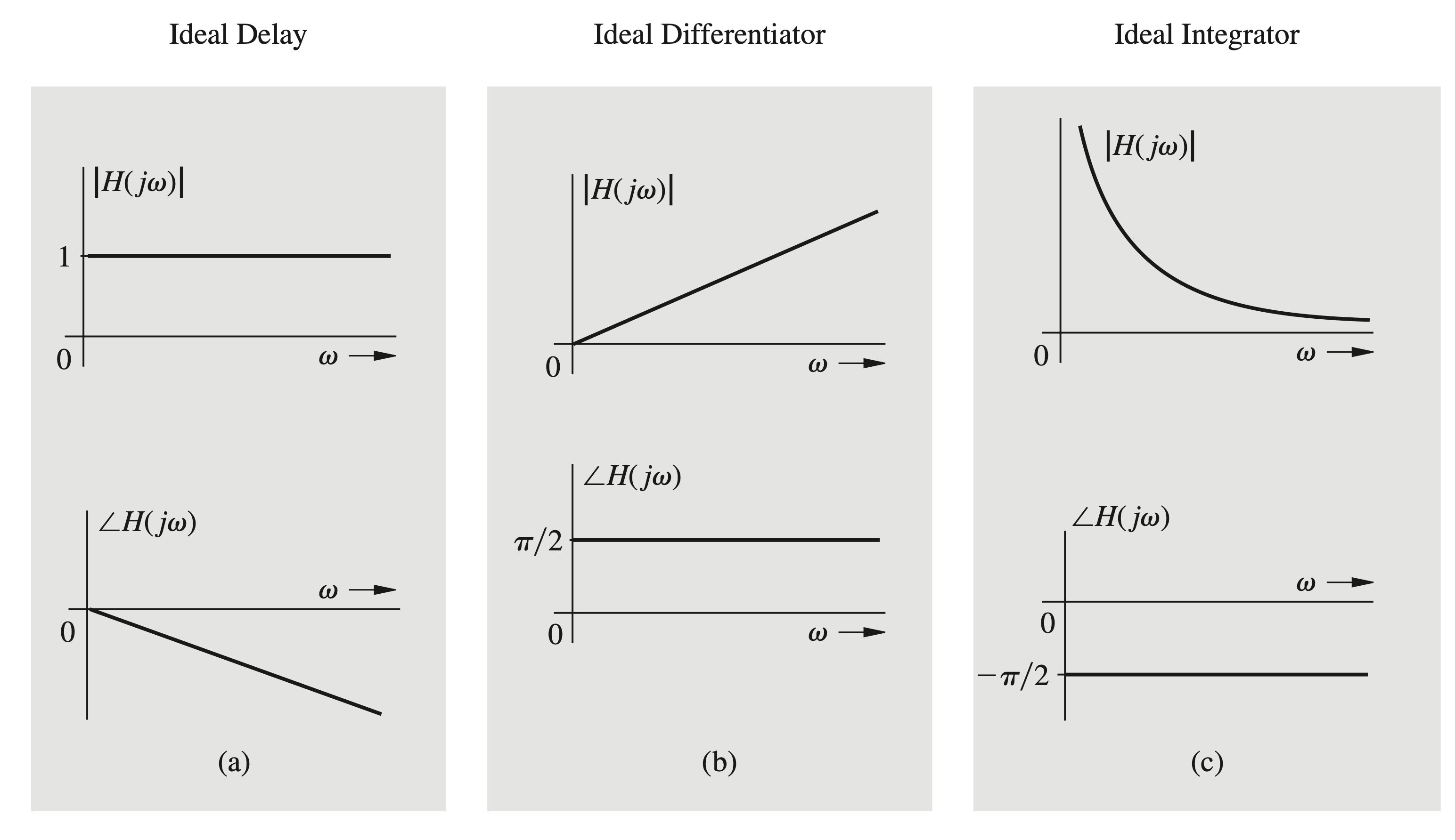
These amplitude and phase responses are shown in Fig. 4.39a. The amplitude response is constant (unity) for all frequencies. The phase shift increases linearly with frequency with a slope of $-T$. This result can be explained physically by recognizing that if a sinusoid $\cos \omega t$ is passed through an ideal delay of $T$ seconds, the output is $\cos \omega (t-T)$. The output sinusoid amplitude is the same as that of the input for all values of $\omega$. Therefore, the amplitude response (gain) is unity for all frequencies. Moreover, the output $\cos \omega (t-T)=\cos (\omega t-\omega T)$ has a phase shift $-\omega T$ with respect to the input $\cos \omega t$. Therefore, the phase response is linearly proportional to the frequency $\omega$ with a slope $-T$.

(b) Ideal differentiator

The transfer function of an ideal differentiator is (see -->here) $$H(s)=s$$

Therefore, $$H(j\omega )=j\omega =\omega e^{j\pi /2}$$

Consequently, $$|H(j\omega )|=\omega \text{ and }\mathrm{\angle }H(j\omega )=\frac{\pi }{2}$$

These amplitude and phase responses are depicted in Fig. 4.39b. The amplitude response increases linearly with frequency, and phase response is constant $(\pi /2)$ for all frequencies. This result can be explained physically by recognizing that if a sinusoid $\cos \omega t$ is passed through an ideal differentiator, the output is $-\omega \sin \omega t=\omega \cos [\omega t+(\pi /2)]$. Therefore, the output sinusoid amplitude is $\omega$ times the input amplitude; that is, the amplitude response (gain) increases linearly with frequency $\omega$. Moreover, the output sinusoid undergoes a phase shift $\pi /2$ with respect to the input $\cos \omega t$. Therefore, the phase response is constant ( $\pi /2)$ with frequency.

In an ideal differentiator, the amplitude response (gain) is proportional to frequency $[|H(j\omega )|=\omega ]$ so that the higher-frequency components are enhanced (see Fig. 4.39b). All practical signals are contaminated with noise, which, by its nature, is a broadband (rapidly varying) signal containing components of very high frequencies. A differentiator can increase the noise disproportionately to the point of drowning out the desired signal. This is why ideal differentiators are avoided in practice.

(c) ideal integrator

The transfer function of an ideal integrator is (see -->here) $$H(s)=\frac{1}{s}$$

Therefore, $$H(j\omega )=\frac{1}{j\omega }=\frac{-j}{\omega }=\frac{1}{\omega }{e}^{-j\pi /2}$$

Consequently, $$|H(j\omega )|=\frac{1}{\omega }\text{ and }\mathrm{\angle }H(j\omega )=-\frac{\pi }{2}$$

These amplitude and phase responses are illustrated in Fig. 4.39c. The amplitude response is inversely proportional to frequency, and the phase shift is constant $(-\pi /2)$ with frequency. This result can be explained physically by recognizing that if a sinusoid $\cos \omega t$ is passed through an ideal integrator, the output is $(1/\omega )\sin \omega t=(1/\omega )\cos [\omega t-(\pi /2)]$. Therefore, the amplitude response is inversely proportional to $\omega$, and the phase response is constant ( $-\pi /2)$