Filter Design by Placement of Poles and Zeros of the Transfer Function

Sources:

1. B. P. Lathi & Roger Green. (2018). Chapter 4: The Laplace Transform. Signal Processing and Linear Systems (3rd ed., pp. 436-445). Oxford University Press.

In this section we explore the strong dependence of frequency response on the location of poles and zeros of $H(s)$. This dependence points to a simple intuitive procedure to filter design.

Dependence of frequency response on poles and zeros of $H(s)$

Frequency response of a system is basically the information about the filtering capability of the system. A system transfer function can be expressed as $$H(s)=\frac{P(s)}{Q(s)}=b_0\frac{(s-z_1)(s-z_2)\cdots (s-z_N)}{(s-{\lambda }_1)(s-{\lambda }_2)\cdots (s-{\lambda }_N)}$$ where $z_1,z_2,\dots ,z_N$ are ${\lambda }_1,{\lambda }_2,\dots ,{\lambda }_N$ are the poles of $H(s)$. Now the value of the transfer function $H(s)$ at some frequency $s=p$ is $$\begin{array}{rl}& H(s){|}_{s=p}\\ \text{(1)}& =& b_0\frac{(p-z_1)\cdots (p-z_N)}{(p-{\lambda }_1)\cdots (p-{\lambda }_N)}\end{array}$$

This equation consists of factors of the form $p-z_i$ and $p-{\lambda }_i$.

Figure 4.48

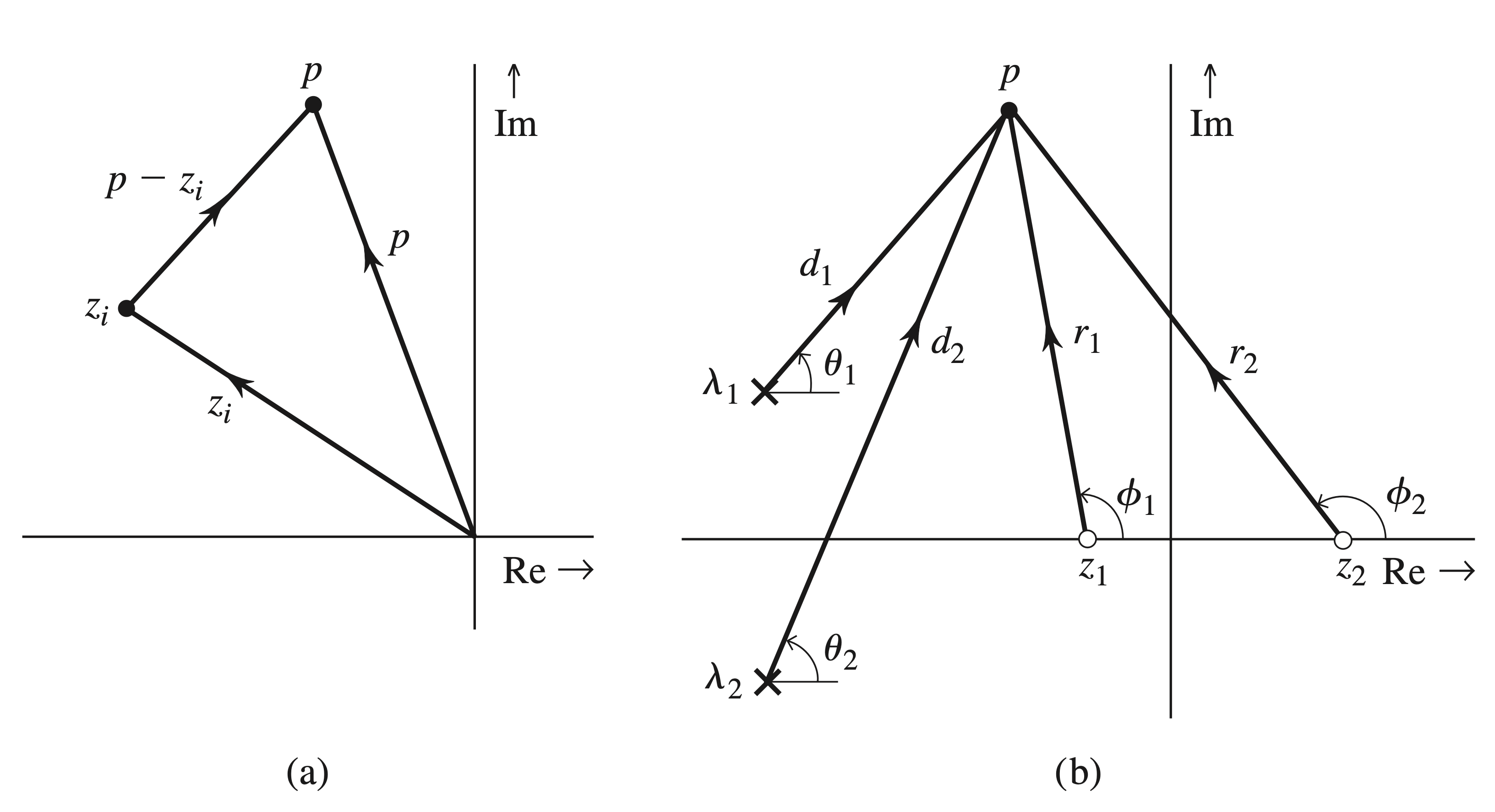
The factor $p-z_i$ is a complex number represented by a vector drawn from point $z$ to the point $p$ in the complex plane, as illustrated in Fig. 4.48a. The length of this line segment is $|p-z_i|$, the magnitude of $p-z_i$.

The angle of this directed line segment (with the horizontal axis) is $\mathrm{\angle }(p-z_i)$. To compute $H(s)$ at $s=p$, we draw line segments from all poles and zeros of $H(s)$ to the point $p$, as shown in Fig. 4.48b.

The vector connecting a zero $z_i$ to the point $p$ is $p-z_i$. Let the length of this vector be $r_i$, and let its angle with the horizontal axis be ${\varphi }_i$. Then $p-z_i=r_i{e}^{j{\varphi }_i}$. Similarly, the vector connecting a pole ${\lambda }_i$ to the point $p$ is $p-{\lambda }_i=d_i{e}^{j{\theta }_i}$, where $d_i$ and ${\theta }_i$ are the length and the angle (with the horizontal axis), respectively, of the vector $p-{\lambda }_i$. Now from Eq. (4.53) it follows that $$\begin{array}{rl}{H(s)|}_{s=p}& =b_0\frac{\left(r_1{e}^{j{\varphi }_1}\right)\left(r_2{e}^{j{\varphi }_2}\right)\cdots \left(r_N{e}^{j{\varphi }_N}\right)}{\left(d_1{e}^{j{\theta }_1}\right)\left(d_2{e}^{j{\theta }_2}\right)\cdots \left(d_N{e}^{j{\theta }_N}\right)}\\ & =b_0\frac{r_1{r}_2\cdots r_N}{d_1{d}_2\cdots d_N}{e}^{j[({\varphi }_1+{\varphi }_2+\cdots +{\varphi }_N)-({\theta }_1+{\theta }_2+\cdots +{\theta }_N)]}\end{array}$$

Therefore $$|H(s){|}_{s=p}=b_0\frac{r_1{r}_2\cdots r_N}{d_1{d}_2\cdots d_N}=b_0\frac{\text{ product of distances of zeros to }p}{\text{ product of distances of poles to }p}$$ and $$\begin{array}{rl}{\mathrm{\angle }H(s)|}_{s=p}& =({\varphi }_1+{\varphi }_2+\cdots +{\varphi }_N)-({\theta }_1+{\theta }_2+\cdots +{\theta }_N)\\ & =\text{ sum of angles of zeros to }p-\text{ sum of angles of poles to }p\end{array}$$

Here, we have assumed positive $b_0$. If $b_0$ is negative, there is an additional phase $\pi$. Using this procedure, we can determine $H(s)$ for any value of $s$.

Gain enhancement by a pole

Figure 4.49

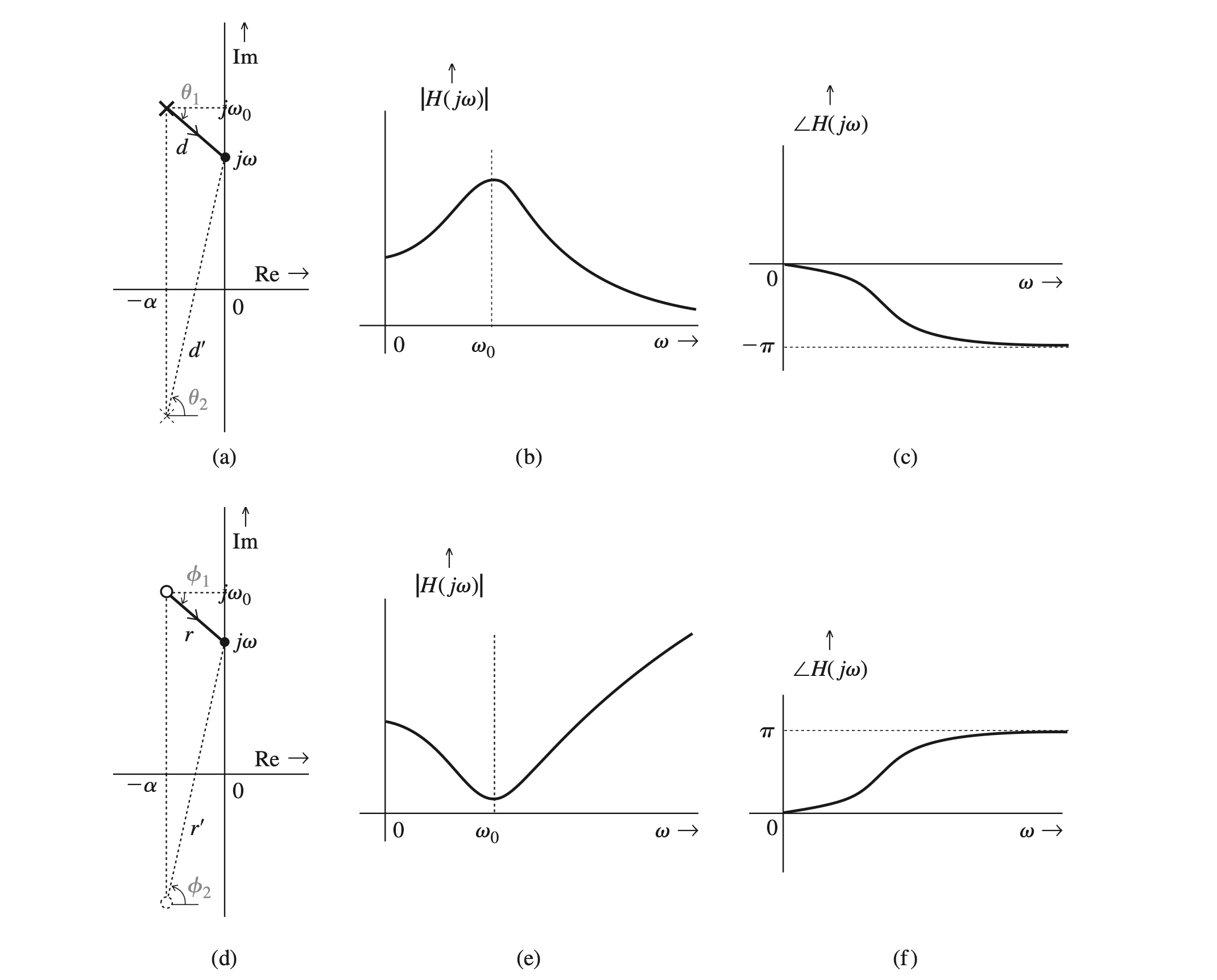
To understand the effect of poles and zeros on the frequency response, consider a hypothetical case of a single pole $-\alpha +j{\omega }_0$, as depicted in Fig. 4.49a. To find the amplitude response $|H(j\omega )|$ for a certain value of $\omega$, we connect the pole to the point $j\omega$ (Fig. 4.49a). If the length of this line is $d$, then $|H(j\omega )|$ is proportional to $1/d$, $$|H(j\omega )|=\frac{K}{d}$$ where the exact value of constant $K$ is not important at this point. As $\omega$ increases from zero, $d$ decreases progressively until $\omega$ reaches the value ${\omega }_0$. As $\omega$ increases beyond ${\omega }_0,d$ increases progressively. Therefore, according to Eq. (4.56), the amplitude response $|H(j\omega )|$ increases from $\omega =0$ until $\omega ={\omega }_0$, and it decreases continuously as $\omega$ increases beyond ${\omega }_0$, as illustrated in Fig. 4.49b. Therefore, a pole at $-\alpha +j{\omega }_0$ results in a frequency-selective behavior that enhances the gain at the frequency ${\omega }_0$ (resonance). Moreover, as the pole moves closer to the imaginary axis (as $\alpha$ is reduced), this enhancement (resonance) becomes more pronounced. This is because $\alpha$, the distance between the pole and $j{\omega }_0$ ( $d$ corresponding to $j{\omega }_0$ ), becomes smaller, which increases the gain $K/d$. In the extreme case, when $\alpha =0$ (pole on the imaginary axis), the gain at ${\omega }_0$ goes to infinity. Repeated poles further enhance the frequency-selective effect. To summarize, we can enhance a gain at a frequency ${\omega }_0$ by placing a pole opposite the point $j{\omega }_0$. The closer the pole is to $j{\omega }_0$, the higher is the gain at ${\omega }_0$, and the gain variation is more rapid (more frequency selective) in the vicinity of frequency ${\omega }_0$. Note that a pole must be placed in the LHP for stability.

Here we have considered the effect of a single complex pole on the system gain. For a real system, a complex pole $-\alpha +j{\omega }_0$ must accompany its conjugate $-\alpha -j{\omega }_0$. We can readily show that the presence of the conjugate pole does not appreciably change the frequency-selective behavior in the vicinity of ${\omega }_0$.

This is because the gain in this case is $$K/d{d}^{\prime },$$ where $d^{\prime }$ is the distance of a point $j\omega$ from the conjugate pole $-\alpha -j{\omega }_0$.

Because the conjugate pole is far from $j{\omega }_0$, there is no dramatic change in the length $d^{\prime }$ as $\omega$ varies in the vicinity of ${\omega }_0$. There is a gradual increase in the value of $d^{\prime }$ as $\omega$ increases, which leaves the frequency-selective behavior as it was originally, with only minor changes.

Gain supression by a zero

Using the same argument, we observe that zeros at $-\alpha \pm j{\omega }_0$ (Fig. 4.49d ) will have exactly the opposite effect of suppressing the gain in the vicinity of ${\omega }_0$, as shown in Fig. 4.49e). A zero on the imaginary axis at $j{\omega }_0$ will totally suppress the gain (zero gain) at frequency ${\omega }_0$. Repeated zeros will further enhance the effect. Also, a closely placed pair of a pole and a zero (dipole) tend to cancel out each other's influence on the frequency response. Clearly, a proper placement of poles and zeros can yield a variety of frequency-selective behavior. We can use these observations to design lowpass, highpass, bandpass, and bandstop (or notch) filters.

Lowpass Filters

Figure 4.50

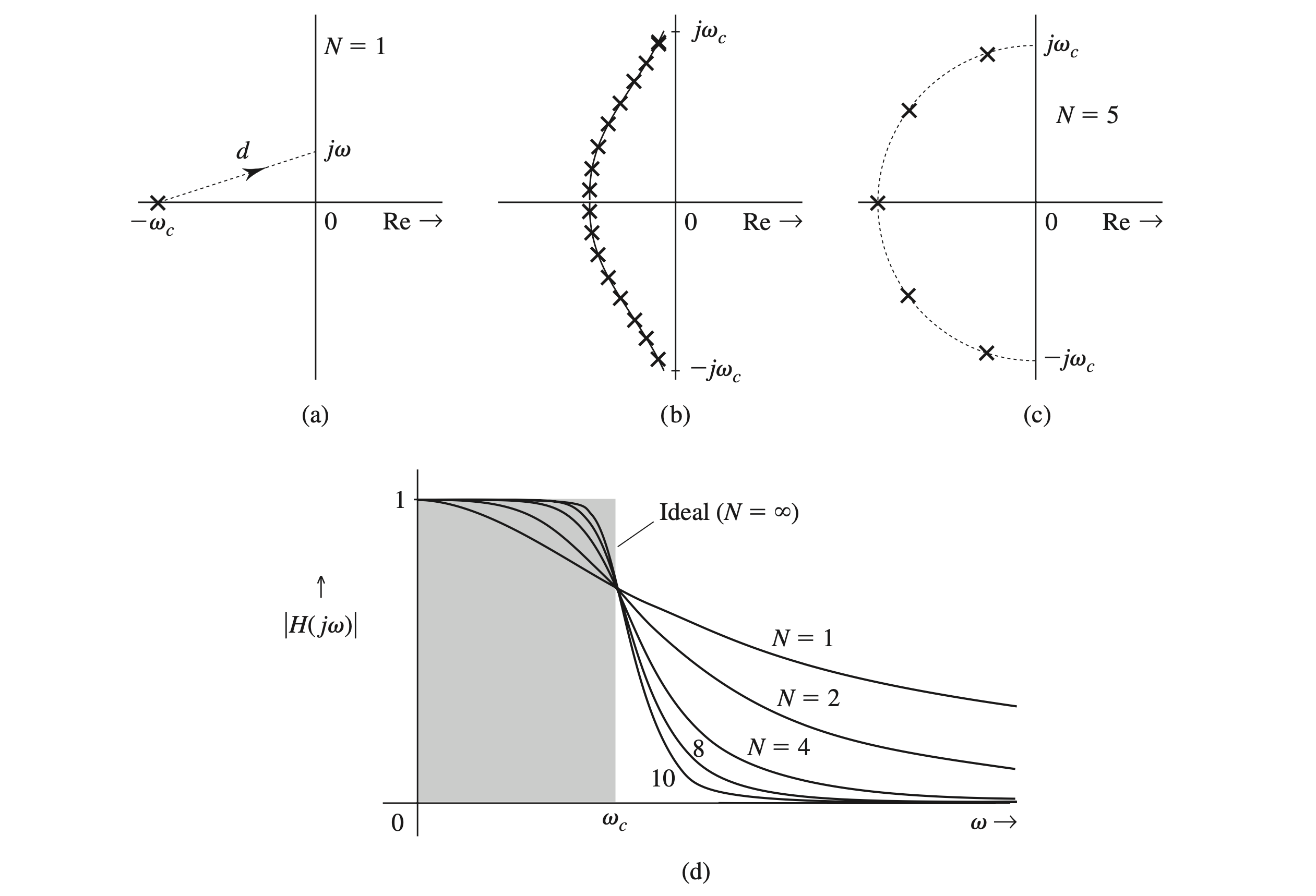
A typical lowpass filter has a maximum gain at $\omega =0$. Because a pole enhances the gain at frequencies in its vicinity, we need to place a pole (or poles) on the real axis opposite the origin $(j\omega =0)$, as shown in Fig. 4.50a. The transfer function of this system is $$H(s)=\frac{{\omega }_c}{s+{\omega }_c}$$

We have chosen the numerator of $H(s)$ to be ${\omega }_c$ to normalize the dc gain $H(0)$ to unity. If $d$ is the distance from the pole $-{\omega }_c$ to a point $j\omega$ (Fig. 4.50a), then $$|H(j\omega )|=\frac{{\omega }_c}{d}$$ with $H(0)=1$. As $\omega$ increases, $d$ increases and $|H(j\omega )|$ decreases monotonically with $\omega$, as illustrated in Fig. 4.50d with label $N=1$. This is clearly a lowpass filter with gain enhanced in the vicinity of $\omega =0$.

Wall of poles

An ideal lowpass filter characteristic (shaded in Fig. 4.50d) has a constant gain of unity up to frequency ${\omega }_c$. Then the gain drops suddenly to 0 for $\omega >{\omega }_c$.

To achieve the ideal lowpass characteristic, we need enhanced gain over the entire frequency band from 0 to ${\omega }_c$. We know that

1. To enhance a gain at any frequency $\omega$, we need to place a pole opposite $\omega$.
2. To achieve an enhanced gain for all frequencies over the band ( 0 to ${\omega }_c$ ), we need to place a pole opposite every frequency in this band.

In other words, we need a continuous wall of poles facing the imaginary axis opposite the frequency band 0 to ${\omega }_c$ (and from 0 to $-{\omega }_c$ for conjugate poles), as depicted in Fig. 4.50b.

At this point, the optimum shape of this wall is not obvious because our arguments are qualitative and intuitive. Yet, it is certain that to have enhanced gain (constant gain) at every frequency over this range, we need an infinite number of poles on this wall.

We can ->show that for a maximally flat response over the frequency range ( 0 to ${\omega }_c$ ), the wall is a semicircle with an infinite number of poles uniformly distributed along the wall.

In practice, we compromise by using a finite number $(N)$ of poles with less-than-ideal characteristics. Figure 4.50c shows the pole configuration for a fifth-order $(N=5)$ filter. The amplitude response for various values of $N$ is illustrated in Fig. 4.50d. As $N\to \mathrm{\infty }$, the filter response approaches the ideal.

This family of filters is known as the Butterworth filters. There are other families of filters, such as the Chebyshev filters. Foe details of this part, see my post about practical filters.

Bandpass Filters

Figure4.51

The shaded characteristic in Fig. 4.51b shows the ideal bandpass filter gain. In the bandpass filter, the gain is enhanced over the entire passband. Our earlier discussion indicates that this can be realized by a wall of poles opposite the imaginary axis in front of the passband centered at ${\omega }_0$. (There is also a wall of conjugate poles opposite $-{\omega }_0$.) Ideally, an infinite number of poles is required. In practice, we compromise by using a finite number of poles and accepting less-than-ideal characteristics (Fig. 4.51). # Notch (Bandstop) Filters

Figure 4.52

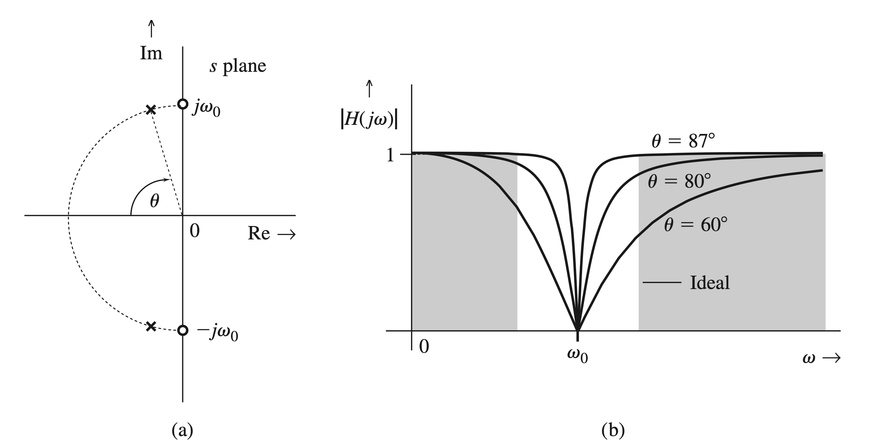
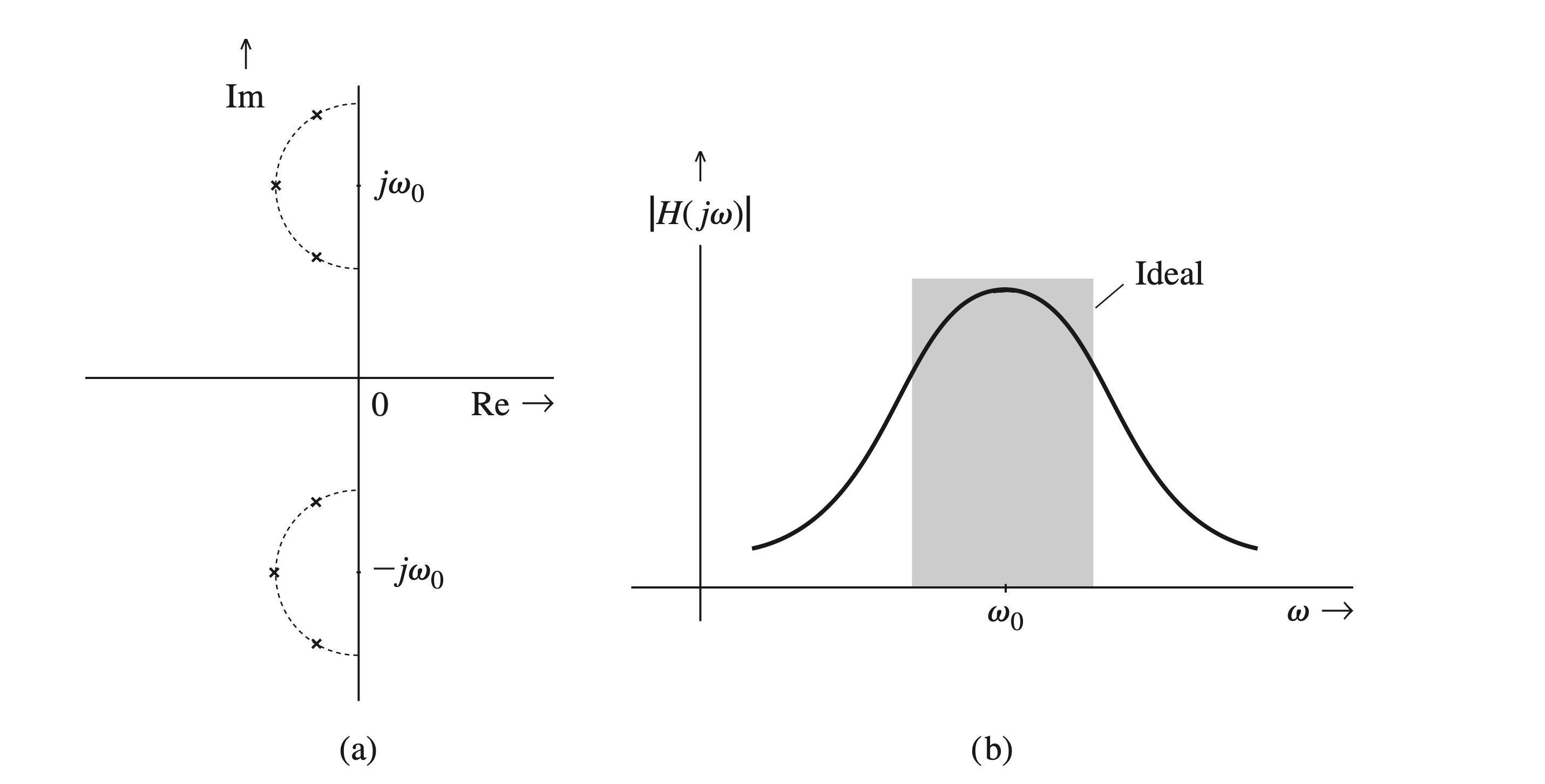
An ideal notch filter amplitude response (shaded in Fig. 4.52b) is a complement of the amplitude response of an ideal bandpass filter. Its gain is zero over a small band centered at some frequency ${\omega }_0$ and is unity over the remaining frequencies. Realization of such a characteristic requires an infinite number of poles and zeros. Let us consider a practical second-order notch filter to obtain zero gain at a frequency $\omega ={\omega }_0$. For this purpose, we must have zeros at $\pm j{\omega }_0$. The requirement of unity gain at $\omega =\mathrm{\infty }$ requires the number of poles to be equal to the number of zeros $(M=N)$. This ensures that for very large values of $\omega$, the product of the distances of poles from $\omega$ will be equal to the product of the distances of zeros from $\omega$. Moreover, unity gain at $\omega =0$ requires a pole and the corresponding zero to be equidistant from the origin. For example, if we use two (complex-conjugate) zeros, we must have two poles; the distance from the origin of the poles and of the zeros should be the same. This requirement can be met by placing the two conjugate poles on the semicircle of radius ${\omega }_0$, as depicted in Fig. 4.52a. The poles can be anywhere on the semicircle to satisfy the equidistance condition. Let the two conjugate poles be at angles $\pm \theta$ with respect to the negative real axis. Recall that a pole and a zero in the same vicinity tend to cancel out each other's influences. Therefore, placing poles closer to zeros (selecting $\theta$ closer to $\pi /2$ ) results in a rapid recovery of the gain from value 0 to 1 as we move away from ${\omega }_0$ in either direction. Figure $4.52\mathrm{b}$ shows the gain $|H(j\omega )|$ for three different values of $\theta$.