The Sampling Theorem

Sources:

1. B. P. Lathi & Roger Green. (2018). Chapter 8: Sampling: The Bridge From Continuous To Discrete. Signal Processing and Linear Systems (3rd ed., pp. 775-784). Oxford University Press.

In this article, we show that a real signal $x(t)$ whose spectrum is bandlimited to $B$ Hz, i.e., $X(\omega )=0$ for $|\omega |>2\pi B)$, can be reconstructed exactly (without any error) from its samples taken uniformly at a rate $f_s>2B$ samples per second. In other words, the minimum sampling frequency is $$f_s>2B$$ Hz.

NOTE: In some literature, $f_s=2B$ is be used, which is not correct.

Notation

Symbol	Meaning
$f_s$	The sampling frequency in Hz.
$\overline{x}(t)$	The sampled signal $\overline{x}(t)$ whereas the original signal is $x(t)$.
${\delta }_T(t)$	The impulse train signal, consisting of unit impulses repeating periodically every $T$ seconds,

The sampling theorem

To prove the sampling theorem, consider a signal $x(t)$ (Fig. 8.1a) whose spectrum (Fig. 8.1b) is bandlimited to $B$ Hz.

Figure 8.1

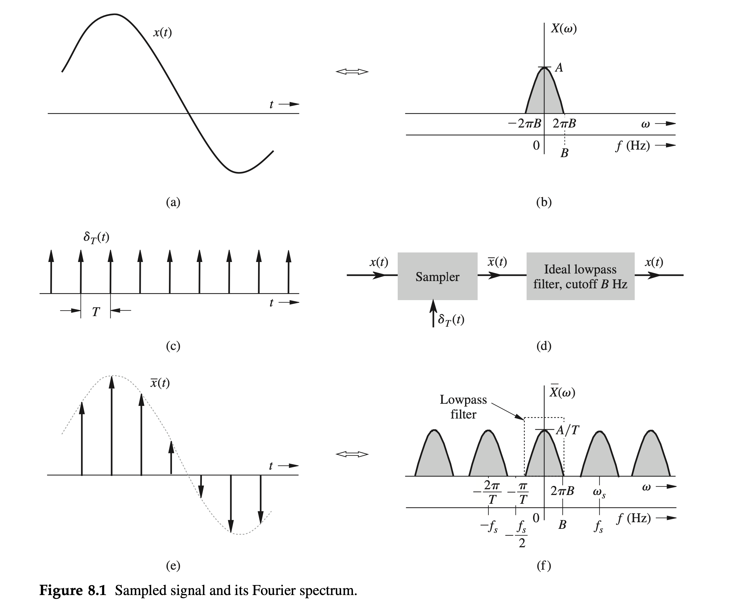
For convenience, spectra are shown as functions of $\omega$ as well as of $f$ (hertz).

Sampling $x(t)$ at a rate of $f_s$ Hz can be accomplished by multiplying $x(t)$ by an impulse train ${\delta }_T(t)$ (Fig. 8.1c), consisting of unit impulses repeating periodically every $T$ seconds, where $T=1/f_s$. The schematic of a sampler is shown in Fig. 8.1d. The resulting sampled signal $\overline{x}(t)$ is shown in Fig. 8.1e.

The sampled signal consists of impulses spaced every $T$ seconds (the sampling interval). The $n$th impulse, located at $t=nT$, has a strength $x(nT)$, the value of $x(t)$ at $t=nT$. $$\overline{x}(t)=x(t){\delta }_T(t)=\sum _{n}x(nT)\delta (t-nT)$$

Because the impulse train ${\delta }_T(t)$ is a periodic signal of period $T$, it can be expressed as a trigonometric Fourier series: $${\delta }_T(t)=\frac{1}{T}[1+2\cos {\omega }_{s}t+2\cos 2{\omega }_{s}t+2\cos 3{\omega }_{s}t+\cdots ]{\omega }_s=\frac{2\pi }{T}=2\pi f_s$$

Therefore, $$\overline{x}(t)=x(t){\delta }_T(t)=\frac{1}{T}[x(t)+2x(t)\cos {\omega }_{s}t+2x(t)\cos 2{\omega }_{s}t+2x(t)\cos 3{\omega }_{s}t+\cdots ]$$

To find $\overline{X}(\omega )$, the Fourier transform of $\overline{x}(t)$, we take the Fourier transform of the right-hand side of this equation, term by term.

1. The transform of the first term in the brackets is $X(\omega )$.

2. The transform of the second term $2x(t)\cos {\omega }_{s}t$ is $X(\omega -{\omega }_s)+X(\omega +{\omega }_s)$. This represents spectrum $X(\omega )$ shifted to ${\omega }_s$ and $-{\omega }_s$.

3. Similarly, the transform of the third term $2x(t)\cos 2{\omega }_{s}t$ is $X(\omega -2{\omega }_s)+X(\omega +2{\omega }_s)$, which represents the spectrum $X(\omega )$ shifted to $2{\omega }_s$ and $-2{\omega }_s$, and so on to infinity.

This result means that the spectrum $\overline{X}(\omega )$ consists of $X(\omega )$ repeating periodically with period ${\omega }_s=2\pi /T\mathrm{rad}/\mathrm{s}$, or $f_s=1/T\mathrm{Hz}$, as depicted in Fig. 8.1f. Therefore,

$$\overline{X}(\omega )=\frac{1}{T}\sum _{n=-\mathrm{\infty }}^{\mathrm{\infty }}X(\omega -n{\omega }_s)$$

If we are to reconstruct $x(t)$ from $\overline{x}(t)$, we should be able to recover $X(\omega )$ from $\overline{X}(\omega )$. This recovery is possible if there is no overlap between successive cycles of $\overline{X}(\omega )$. Figure 8.1f indicates that this requires $$\begin{array}{}\text{(1)}& f_s>2B\end{array}$$

Also, the sampling interval $T=1/f_s$. Therefore, $$T<\frac{1}{2B}$$

The corresponding sampling interval $T=1/2B$ is called the Nyquist interval for $x(t)$.

Thus, as long as the sampling frequency $f_s>2B$ (in hertz), $\overline{X}(\omega )$ consists of nonoverlapping repetitions of $X(\omega )$, and $x(t)$ can be recovered from its samples $\overline{x}(t)$ by passing the sampled signal $\overline{x}(t)$ through an ideal lowpass filter having a bandwidth of any value between $B$ and $f_s-B$ Hz.

Practical sampling

In proving the sampling theorem, we assumed ideal samples obtained by multiplying a signal $x(t)$ by an impulse train that is physically unrealizable. In practice, we multiply a signal $x(t)$ by a train of pulses of finite width, depicted in Fig. 8.3c. The sampler is shown in Fig. 8.3d. The sampled signal $\overline{x}(t)$ is illustrated in Fig. 8.3e.

Figure 8.3

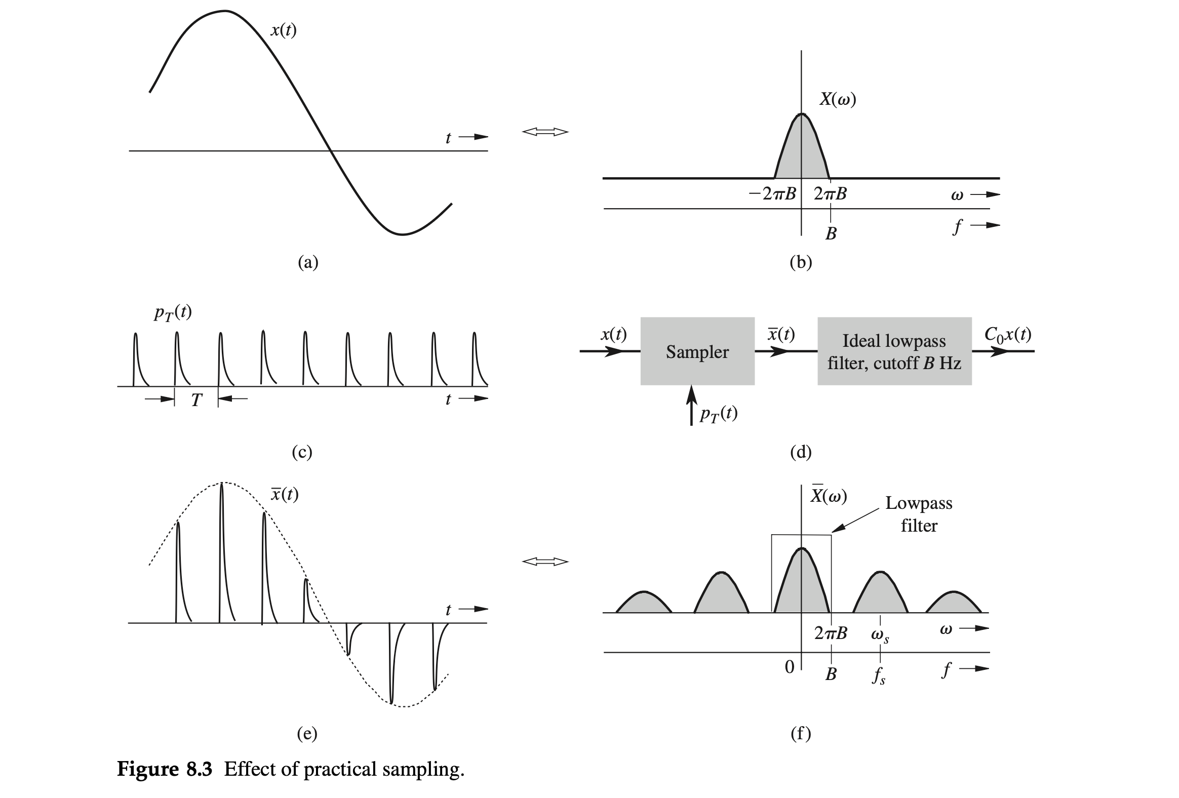
We wonder whether it is possible to recover or reconstruct $x(t)$ from this $\overline{x}(t)$. Surprisingly, the answer is affirmative, provided the sampling rate is not below the Nyquist rate. The signal $x(t)$ can be recovered by lowpass filtering $\overline{x}(t)$ as if it were sampled by impulse train.

The plausibility of this result becomes apparent when we consider the fact that reconstruction of $x(t)$ requires the knowledge of the Nyquist sample values. This information is available or built into the sampled signal $\overline{x}(t)$ in Fig. 8.3e because the $n$th sampled pulse strength is $x(nT)$. To prove the result analytically, we observe that the sampling pulse train $p_T(t)$ depicted in Fig. 8.3c, being a periodic signal, can be expressed as a trigonometric Fourier series $$p_T(t)=C_0+\sum _{n=1}^{\mathrm{\infty }}{C}_n\cos (n{\omega }_{s}t+{\theta }_n){\omega }_s=\frac{2\pi }{T}$$

Thus, $$\begin{array}{rl}\overline{x}(t)& =x(t)p_T(t)=x(t)[C_0+\sum _{n=1}^{\mathrm{\infty }}{C}_n\cos (n{\omega }_{s}t+{\theta }_n)]\\ & =C_{0}x(t)+\sum _{n=1}^{\mathrm{\infty }}{C}_{n}x(t)\cos (n{\omega }_{s}t+{\theta }_n)\end{array}$$

The sampled signal $\overline{x}(t)$ consists of $$C_{0}x(t),C_{1}x(t)\cos ({\omega }_{s}t+{\theta }_1),C_{2}x(t)\cos (2{\omega }_{s}t+{\theta }_2),\dots$$ Note that the first term $C_{0}x(t)$ is the desired signal and all the other terms are modulated signals with spectra centered at $\pm {\omega }_s,\pm 2{\omega }_s,\pm 3{\omega }_s,\dots$, as illustrated in Fig. 8.3f.

Clearly the signal $x(t)$ can be recovered by lowpass filtering of $\overline{x}(t)$, as shown in Fig. 8.3d. As before, it is necessary that ${\omega }_s>4\pi B($ or $f_s>2B)$.