The Laplace Transform
Sources:
- B. P. Lathi & Roger Green. (2018). Chapter 4: The Laplace Transform. Signal Processing and Linear Systems (3rd ed., pp. 330-404). Oxford University Press.
Bilateral Laplace transform
For a signal \(x(t)\), its (bilateral) Laplace transform \(X(s)\) is defined by \[ \begin{equation} \label{eq4_1} X(s) = \color{blue} {\int_{-\infty}^{\infty} } \color{red}{x(t)} \color{green}{e^{-s t}} \, \color{violet}{dt} \end{equation} \]
The signal \(x(t)\) is said to be the inverse Laplace transform of \(X(s)\). It can be shown that \[ \begin{equation} \label{eq4_2} x(t)=\frac{1}{2 \pi j} \color{blue} { \int_{c-j \infty}^{c+j \infty}} \color{red} {X(s)} \color{green}{e^{s t}} \color{violet}{d s} \end{equation} \] where \(c\) is a constant chosen to ensure the convergence of the integral in \(\eqref{eq4_1}\), as explained later. See also [1].
This pair of equations is known as the bilateral Laplace transform pair, where \(X(s)\) is the direct Laplace transform of \(x(t)\) and \(x(t)\) is the inverse Laplace transform of \(X(s)\). Symbolically, \[ X(s)=\mathcal{L}[x(t)] \quad \text { and } \quad x(t)=\mathcal{L}^{-1}[X(s)] \]
Note that \[ \mathcal{L}^{-1}\{\mathcal{L}[x(t)]\}=x(t) \quad \text { and } \quad \mathcal{L}\left\{\mathcal{L}^{-1}[X(s)]\right\}=X(s) \] It is also common practice to use a bidirectional arrow to indicate a Laplace transform pair, as follows: \[ x(t) \Longleftrightarrow X(s) \]
The term bilateral (or two-sided) comes from the fact that the bilateral Laplace transform can handle signals existing over the entire time interval from \(-\infty\) to \(\infty\).
Later we shall consider a special case-the unilateral or one-sided Laplace transform-which can handle only signals existing from \(t=0\).
In my other post, I will show that any bilateral transform can be expressed in terms of two unilateral transforms.
Region of convergence
The region of convergence (ROC), also called the region of existence, for the Laplace transform, \(X(s)\), is the domain of \(X(s)\), i.e., it is the set of values of \(s\) (the region in the complex plane) for which the integral in \(\eqref{eq4_1}\) converges. For \(s\) outside of ROC, \(\eqref{eq4_1}\) does not converge, so \(X(s)\) is meaningless.
Example
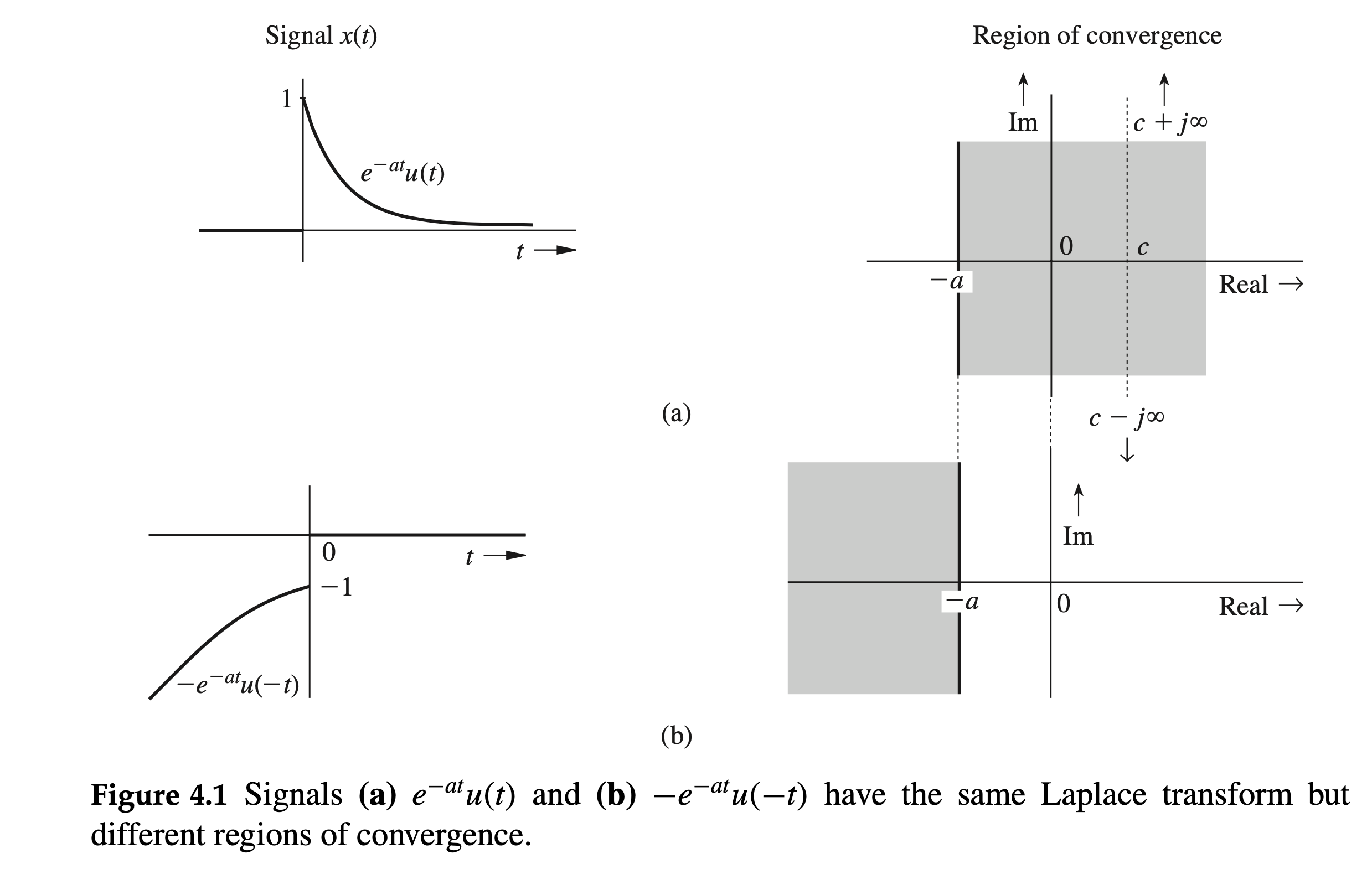
For a signal \(x(t)=e^{-a t} u(t)\), find the Laplace transform \(X(s)\) and its ROC.
By definition, \[ X(s)=\int_{-\infty}^{\infty} e^{-a t} u(t) e^{-s t} d t \]
Because \(u(t)=0\) for \(t<0\) and \(u(t)=1\) for \(t \geq 0\), \[ \begin{align} X(s) & =\int_0^{\infty} e^{-a t} e^{-s t} d t \nonumber \\ & = \int_0^{\infty} e^{-(s+a) t} d t \nonumber \\ & = -\left.\frac{1}{s+a} e^{-(s+a) t}\right|_0 ^{\infty} \label{eq4_4} . \end{align} \] Note that \(s\) is complex and as \(t \rightarrow \infty\), the term \(e^{-(s+a) t}\) does not necessarily vanish. Here we recall that for a complex number \(z=\alpha+j \beta\), \[ e^{-z t}=e^{-(\alpha+j \beta) t}=e^{-\alpha t} e^{-j \beta t} . \]
Now \(\left|e^{-j \beta t}\right|=1\) regardless of the value of \(\beta t\). Therefore, as \(t \rightarrow \infty, e^{-z t} \rightarrow 0\) only if \(\alpha>0\), and \(e^{-z t} \rightarrow \infty\) if \(\alpha<0\). Thus, \[ \lim _{t \rightarrow \infty} e^{-\color{brown}{z} t}= \begin{cases}0 & \operatorname{Re} z>0 \\ \infty & \operatorname{Re} z<0\end{cases} \]
Clearly, \[ \lim _{t \rightarrow \infty} e^{-\color{brown}{(s+a)} t}= \begin{cases}0 & \operatorname{Re}(s+a)>0 \\ \infty & \operatorname{Re}(s+a)<0\end{cases} \]
Use of this result in \(\eqref{eq4_4}\) yields \[ X(s)=\frac{1}{s+a} \quad \operatorname{Re}(s+a)>0 \] or \[ \begin{equation} \label{eq4_6} e^{-a t} u(t) \Longleftrightarrow \frac{1}{s+a} \quad \operatorname{Re} s>-a \end{equation} \]
The ROC of \(X(s)\) is \(\operatorname{Re} s>-a\), as shown in the shaded area in Fig. 4.1a.
Extension of the example
Now, let us find the Laplace transform of signal \(x(t)\) illustrated in Fig. 4.1b: \[ x(t)=-e^{-a t} u(-t) \]
The Laplace transform of this signal is \[ X(s)=\int_{-\infty}^{\infty}-e^{-a t} u(-t) e^{-s t} d t \]
Because \(u(-t)=1\) for \(t<0\) and \(u(-t)=0\) for \(t>0\), \[ X(s)=\int_{-\infty}^0-e^{-a t} e^{-s t} d t=-\int_{-\infty}^0 e^{-(s+a) t} d t=\left.\frac{1}{s+a} e^{-(s+a) t}\right|_{-\infty} ^0 \] We also know that \[ \lim _{t \rightarrow-\infty} e^{-(s+a) t}=0 \quad \operatorname{Re}(s+a)<0 \]
Hence, \[ X(s)=\frac{1}{s+a} \quad \operatorname{Re} s<-a \]
The signal \(-e^{-a t} u(-t)\) and its ROC \((\operatorname{Re} s<-a)\) are depicted in Fig. 4.1b.
Note that the Laplace transforms for the signals \(e^{-a t} u(t)\) and \(-e^{-a t} u(-t)\) are identical except for their regions of convergence. Therefore, for a given \(X(s)\), there may be more than one inverse transform, depending on the ROC. In other words, unless the ROC is specified, there is no one-to-one correspondence between \(X(s)\) and \(x(t)\).
This fact increases the complexity in using the Laplace transform. As a result, people invented the unilateral Laplace transform (# TODO) which only cares about the \(t>0\) part of \(x(t)\), and there is only one inverse transform for a unilateral Laplace transformed function \(X(s)\).
Unilateral Laplace transform
The unilateral Laplace transform is a special case of the bilateral Laplace transform in which we restrict \(x(t)\) to start from \(t=0\), leading to some favorable properties of the transformed function \(X(s)\).
Unless otherwise specified, the term Laplace transform essentially means the unilateral Laplace transform.
The unilateral Laplace transform \(X(s)\) of a signal \(x(t)\) is defined as \[ X(s)=\color{blue} {\int_{0^{-}}^{\infty} } \color{red}{x(t)} \color{green}{e^{-s t}} \, \color{violet}{dt} \]
The inverse Laplace transform for the inilateral Laplace transform remains unchanged.
Note:
- Since the inverse transform of the unilateral Laplace transform is unique, there is no need to specify the ROC explicitly.
Existence of the Laplace transform
The variable \(s\) in the Laplace transform is complex in general, and it can be expressed as \(s=\sigma+j \omega\). By definition, \[ X(s)=\int_{0^{-}}^{\infty} x(t) e^{-s t} d t=\int_{0^{-}}^{\infty}\left[x(t) e^{-\sigma t}\right] e^{-j \omega t} d t \]
Because \(\left|e^{j \omega t}\right|=1\), the integral on the right-hand side of this equation converges if (#TODO the X(s) is a complex integral) \[ \begin{equation} \label{eq4_8} \int_{0^{-}}^{\infty}\left|x(t) e^{-\sigma t}\right| d t<\infty \end{equation} \]
Hence the existence of the Laplace transform is guaranteed if the integral in \(\eqref{eq4_8}\) is finite for some value of \(\sigma\).
One kind of such signals satisfying the condition of \(\eqref{eq4_8}\) is the signals that grow no faster than an exponential signal \(M e^{\sigma_0 t}\) for some \(M\) and \(\sigma_0\). Thus, if for some \(M\) and \(\sigma_0\), \[ |x(t)| \leq M e^{\sigma_0 t}, \] we can choose \(\sigma>\sigma_0\) to satisfy \(\eqref{eq4_8}\)[^1]. The signal \(e^{t^2}\), in contrast, grows at a rate faster than \(e^{\sigma_0 t}\), and consequently is not Laplace-transformable. Fortunately such signals (which are not Laplace-transformable) are of little consequence from either a practical or a theoretical viewpoint.
If \(\sigma_0\) is the smallest value of \(\sigma\) for which the integral in \(\eqref{eq4_8}\) is finite, \(\sigma_0\) is called the abscissa of convergence and the ROC of \(X(s)\) is \[ \color{violet} {\operatorname{Re} s>\sigma_0} . \]
One common signal is \(x(t) = e^{-a t} u(t)\), its abscissa of convergence is \(-a\), and its ROC is \[ \operatorname{Re} s>-a . \]