Sources:

1. B. P. Lathi & Roger Green. (2018). Chapter 4: The Laplace Transform. Signal Processing and Linear Systems (3rd ed., pp. 386-401). Oxford University Press.

Block Diagrams of Systems

Figure 4.18a shows a block diagram of a system with a transfer function $H(s)$ and its input and output $X(s)$ and $Y(s)$. respectively.

Figure 4.18a

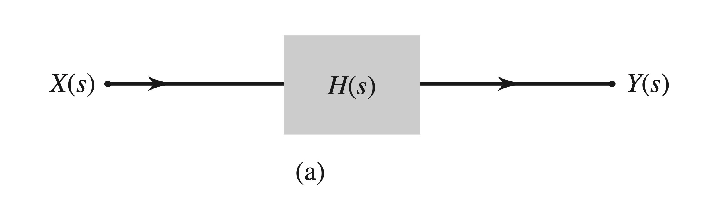
Large systems can be represented by suitably interconnected subsystems, each of which can be readily analyzed. Each subsystem can be characterized in terms of its input–output relationships.

Subsystems may be interconnected by using:

1. cascade,
2. parallel, and
3. feedback

interconnections.

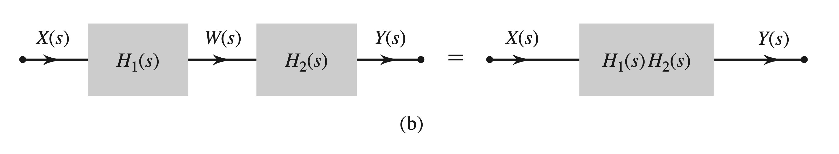
The cascade case

When transfer functions appear in cascade, as depicted in Fig. 4.18b, the transfer function of the overall system is the product of the two transfer functions. $$\frac{Y(s)}{X(s)}=\frac{W(s)}{X(s)}\frac{Y(s)}{W(s)}=H_1(s)H_2(s)$$

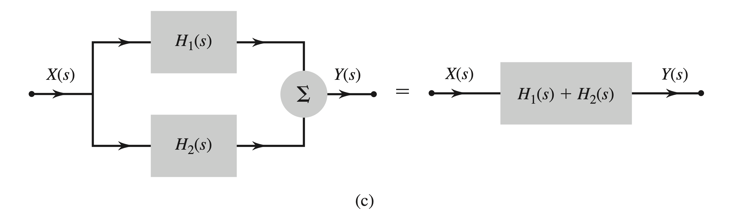
The parallel case

Similarly, when two transfer functions, $H_1(s)$ and $H_2(s)$, appear in parallel, as illustrated in Fig. 4.18c, the overall transfer function is given by $H_1(s)+H_2(s)$.

Figure 4.18c

The feedback (or closed-loop) case

As introduced in a previous post, control systems can be classified into two main types:

1. Open-Loop Systems: These systems operate without feedback, as illustrated in Fig. 4.33a.
2. Closed-Loop Systems: These systems utilize feedback, as illustrated in Fig. 4.33b.

Fig. 4.33a and Fig. 4.33b

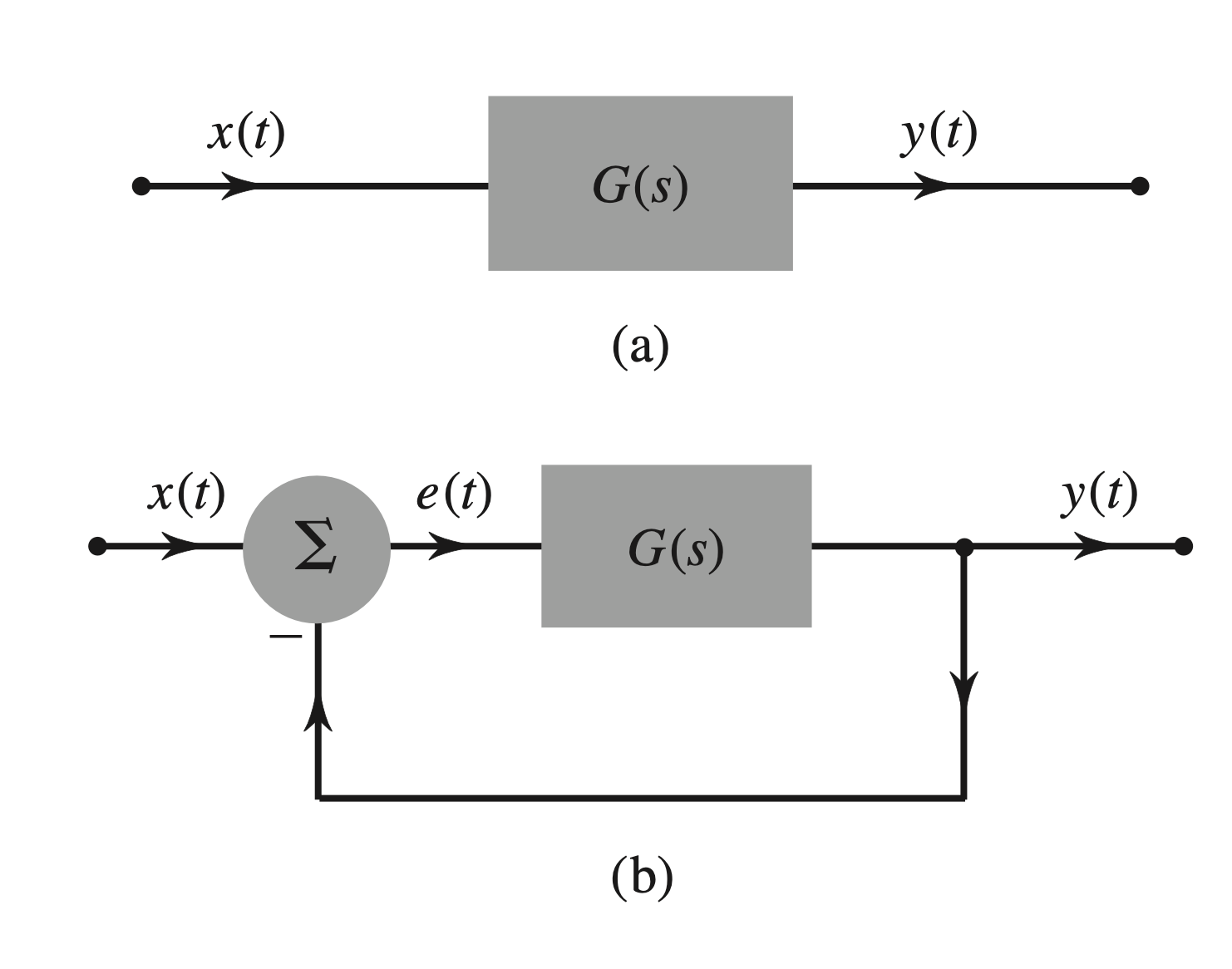
A closed-loop system is also referred to as a feedback system because the output is fed back into the input for control purposes. The overall transfer function $T(s)$ of a feedback system is given by:

$$T(s)=\frac{Y(s)}{X(s)}=\frac{G(s)}{1+G(s)H(s)},$$ where: - $G(s)$ is the forward path transfer function, - $H(s)$ is the feedback path transfer function.

This relationship is illustrated in Fig. 4.18d.

Fig. 4.18d

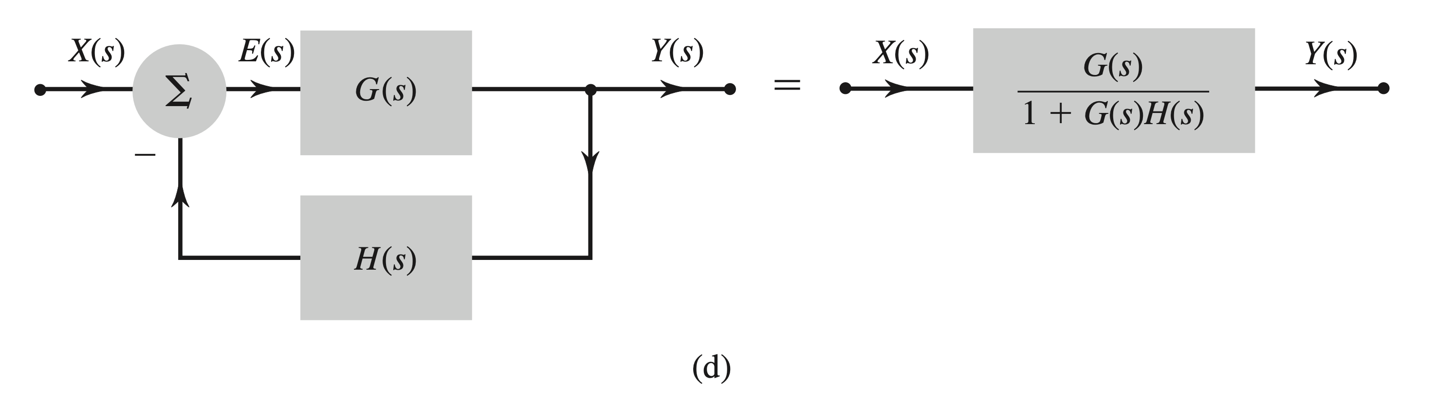
Proof of the feedback transfer function

To derive the transfer function of a feedback system, consider the block diagram shown in Fig. 4.18d. 1. Adder Output:

The inputs to the adder are $X(s)$ and $-H(s)Y(s)$. The output of the adder, $E(s)$, is:

$$E(s)=X(s)-H(s)Y(s)$$

2. Output Relationship:

The output $Y(s)$ is related to $E(s)$ through the forward path transfer function $G(s)$ :

$$Y(s)=G(s)E(s)$$

Substituting $E(s)=X(s)-H(s)Y(s)$ into this equation:

$$Y(s)=G(s)[X(s)-H(s)Y(s)]$$

3. Rearranging Terms:

Expanding and rearranging terms gives:

$$Y(s)[1+G(s)H(s)]=G(s)X(s)$$

4. Transfer Function:

Solving for $\frac{Y(s)}{X(s)}$, the transfer function of the feedback system is:

$$\frac{Y(s)}{X(s)}=\frac{G(s)}{1+G(s)H(s)}$$

This concludes the derivation of the feedback system's transfer function.