The Fourier Transform of Common Functions

Sources:

B. P. Lathi & Roger Green. (2018). Chapter 7: Continuous-Time Signal Analysis. Signal Processing and Linear Systems (3nd ed., pp. 689-701). Oxford University Press.

For convenience, we now introduce a compact notation for the useful gate, triangle, and interpolation functions.

For more results, refer to Table of the Fourier Transform Pairs.

Some common functions

For convenience, we now introduce a compact notation for the useful gate, triangle, and interpolation functions.

Unit gate function

Figure 7.7

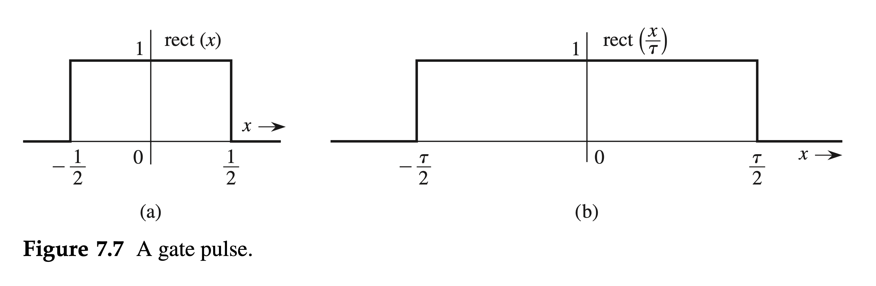
The unit gate function $\mathrm{rect}(x)$ is defined as $$\mathrm{rect}(x)=\{\begin{array}{ll}0& |x|>\frac{1}{2}\\ \frac{1}{2}& |x|=\frac{1}{2}\\ 1& |x|<\frac{1}{2}\end{array},$$

as illustrated in Fig. 7.7a¹.

From this definition, we also have $\mathrm{rect}(x/\tau )$, which is a $\mathrm{rect}(x)$ expanded by a factor $\tau$ along the horizontal axis. This is illustrated in Fig. 7.7b. Observe that $\tau$ indicates the width of the pulse.

Unit triangle function

Figure 7.8

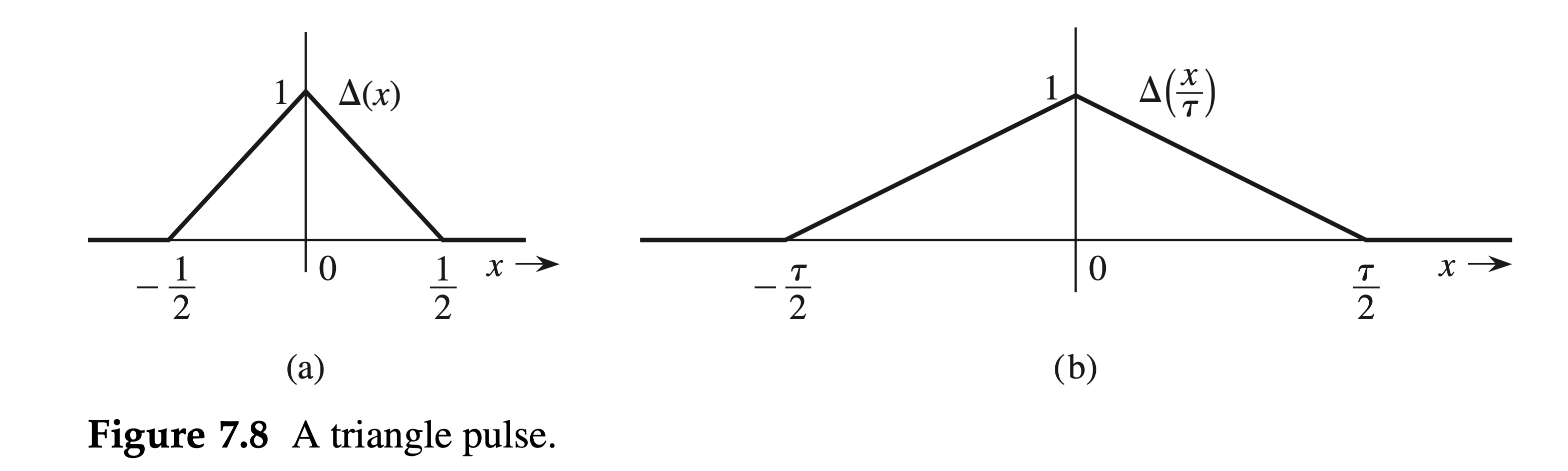
The unit triangle function $\mathrm{\Delta }(x)$ is defined as $$\mathrm{\Delta }(x)=\{\begin{array}{ll}0& |x|\ge \frac{1}{2}\\ 1-2|x|& |x|<\frac{1}{2}\end{array},$$ as illustrated in Fig. 7.8a.

From this definition, we also have $\mathrm{\Delta }(x/\tau )$. This is illustrated in Fig. 7.8b. Observe that $\tau$ indicates the width of the pulse.

Interpolation function

Figure 7.9

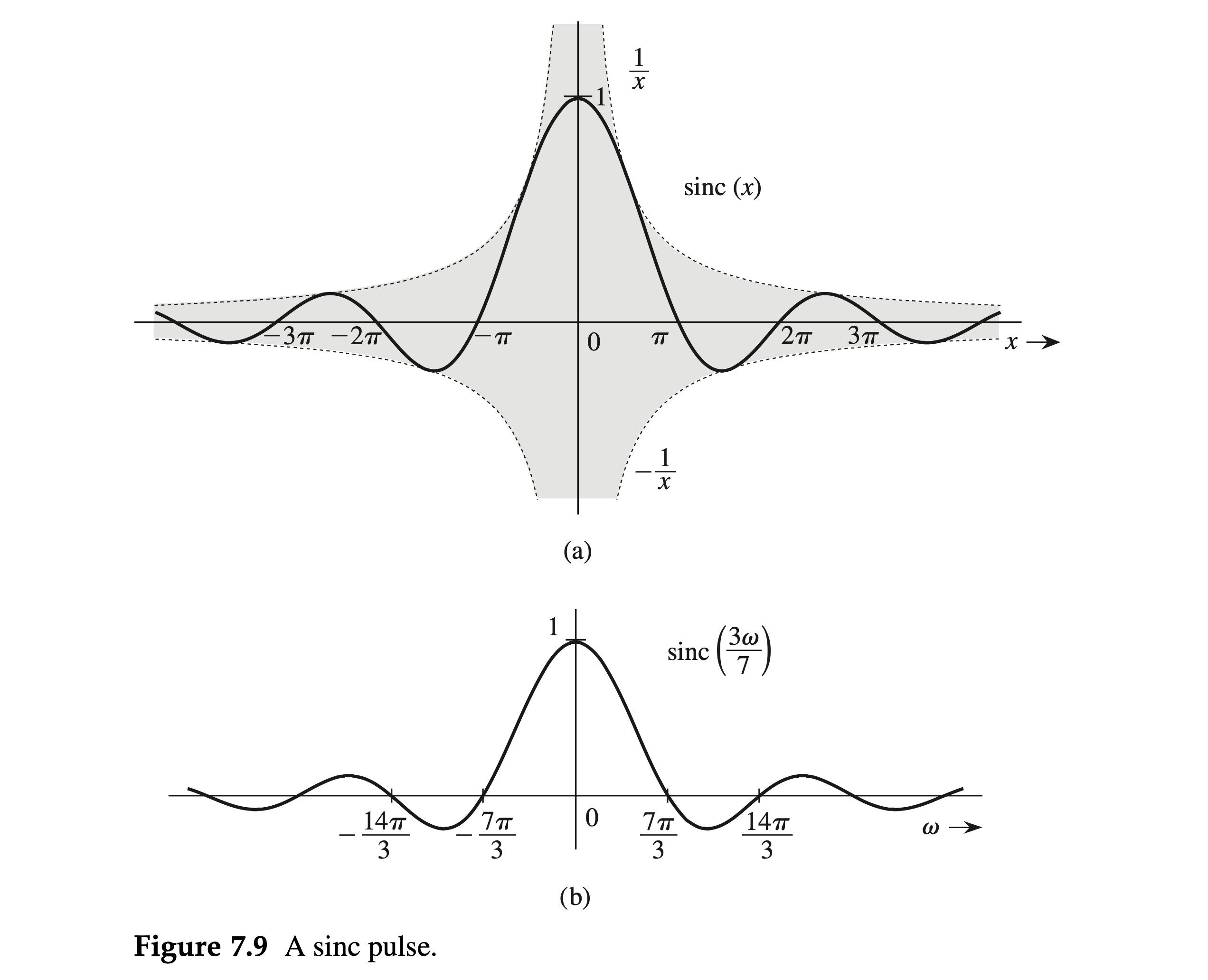
The function $\sin x/x$ plays an important role in signal processing. It is also known as the filtering or interpolating function. We define $$\begin{array}{}\text{(1)}& \mathrm{sinc}(x)=\frac{\sin x}{x}\end{array}$$

Figure 7.9a shows $\mathrm{sinc}(x)$. Figure 7.9b shows $\mathrm{sinc}(3\omega /7)$.

Inspection of $\text{(1)}$ shows the following:

1. $\mathrm{sinc}(x)$ is an even function of $x$.
2. $\mathrm{sinc}(x)=0$ when $\sin x=0$ except at $x=0$, where it appears to be indeterminate. This means that $\mathrm{sinc}x=0$ for $x=\pm \pi ,\pm 2\pi ,\pm 3\pi ,\dots$
3. Using L'Hôpital's rule, we find $\mathrm{sinc}(0)=1$.
4. $\mathrm{sinc}(x)$ is the product of an oscillating signal $\sin x$ (of period $2\pi )$ and a monotonically decreasing function $1/x$. Therefore, $\mathrm{sinc}(x)$ exhibits damped oscillations of period $2\pi$, with amplitude decreasing continuously as $1/x$.

Fourier Transform of a Rectangular Pulse

Figure 7.10

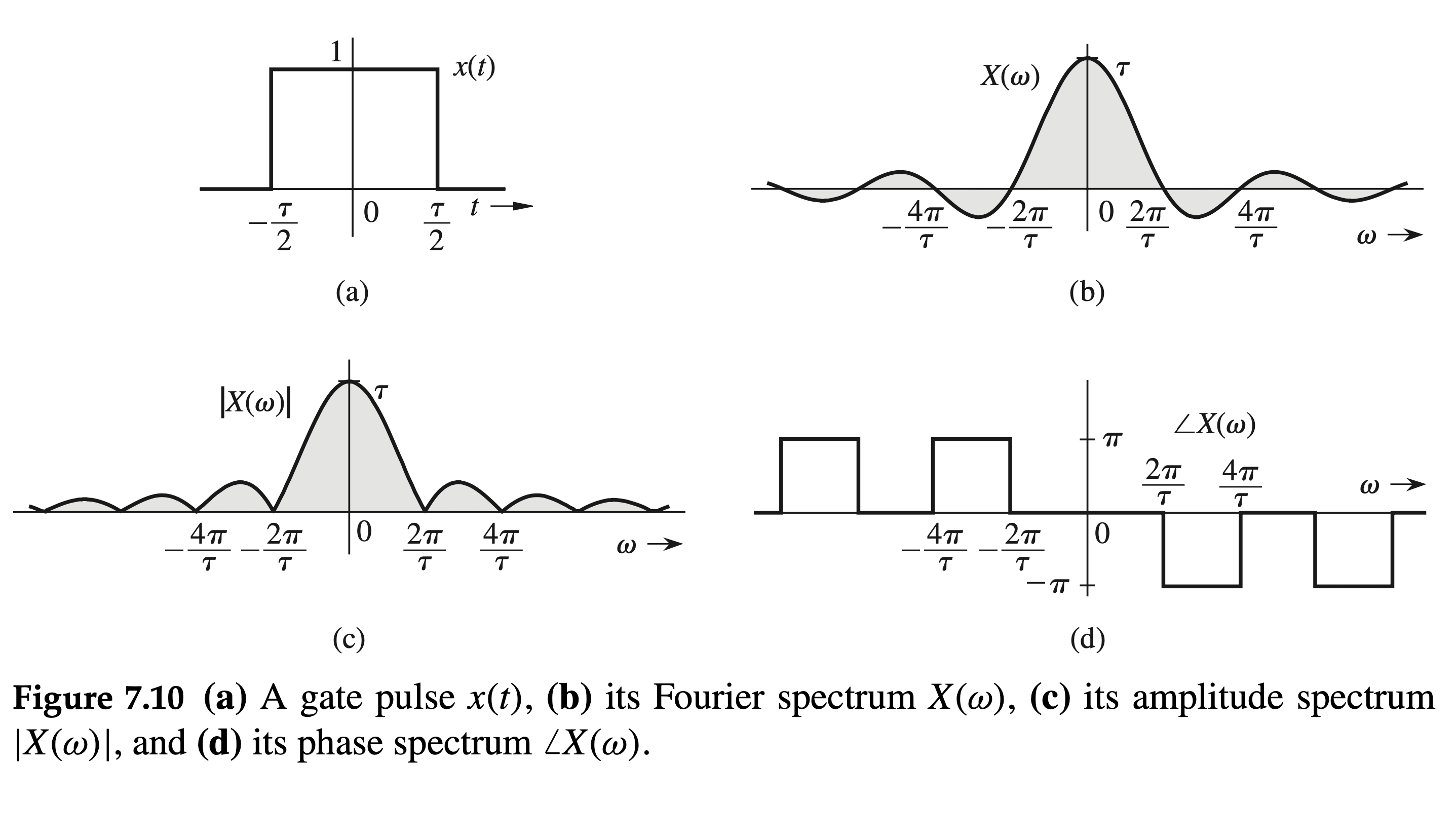
Find the Fourier transform of $x(t)=\mathrm{rect}(t/\tau )$ (Fig. 7.10a). $$X(\omega )={\int }_{-\mathrm{\infty }}^{\mathrm{\infty }}\mathrm{rect}\left(\frac{t}{\tau }\right)e^{-j\omega t}dt$$

Solution:

Since rect $(t/\tau )=1$ for $|t|<\tau /2$, and since it is zero for $|t|>\tau /2$, $$\begin{array}{rl}X(\omega )& ={\int }_{-\tau /2}^{\tau /2}{e}^{-j\omega t}dt\\ & =-\frac{1}{j\omega }(e^{-j\omega \tau /2}-e^{j\omega \tau /2})=\frac{2\sin \left(\frac{\omega \tau }{2}\right)}{\omega }\\ & =\tau \frac{\sin \left(\frac{\omega \tau }{2}\right)}{\left(\frac{\omega \tau }{2}\right)}=\tau \mathrm{sinc}\left(\frac{\omega \tau }{2}\right)\end{array}$$ Therefore, $$\mathrm{rect}\left(\frac{t}{\tau }\right)⟺\tau \mathrm{sinc}\left(\frac{\omega \tau }{2}\right)$$

Recall that $\mathrm{sinc}(x)=0$ when $x=\pm n\pi$. Hence, $\mathrm{sinc}(\omega \tau /2)=0$ when $\omega \tau /2=\pm n\pi$; that is, when $\omega =\pm 2n\pi /\tau ,(n=1,2,3,\dots )$, as depicted in Fig. 7.10b. The Fourier transform $X(\omega )$ shown in Fig. 7.10b exhibits positive and negative values. A negative amplitude can be considered to be a positive amplitude with a phase of $-\pi$ or $\pi$. We use this observation to plot the amplitude spectrum $|X(\omega )|=|\mathrm{sinc}(\omega \tau /2)|$ (Fig. 7.10c) and the phase spectrum $\mathrm{\angle }X(\omega )$ (Fig. 7.10d). The phase spectrum, which is required to be an odd function of $\omega$, may be drawn in several other ways because a negative sign can be accounted for by a phase of $\pm n\pi$, where $n$ is any odd integer. All such representations are equivalent.

Bandwidth of $\text{Missing or unrecognized delimiter for right}$:

The spectrum $X(\omega )$ in Fig. 7.10 peaks at $\omega =0$ and decays at higher frequencies. Therefore, rect $(t/\tau )$ is a lowpass signal with most of the signal energy in lower-frequency components. Strictly speaking, because the spectrum extends from 0 to $\mathrm{\infty }$, the bandwidth is $\mathrm{\infty }$. However, much of the spectrum is concentrated within the first lobe (from $\omega =0$ to $\omega =2\pi /\tau$ ). Therefore, a rough estimate of the bandwidth of a rectangular pulse of width $\tau$ seconds is $2\pi /\tau \mathrm{rad}/\mathrm{s}$, or $1/\tau$ $\mathrm{Hz}{}^{†}$ Note the reciprocal relationship of the pulse width with its bandwidth. We shall observe later that this result is true, in general. To compute bandwidth, we must consider the spectrum for positive values of $\omega$ only. See the discussion in Sec. 6.3.

Fourier Transform of the Dirac Delta Function

Find the Fourier transform of the unit impulse $\delta (t)$.

Figure 7.11

---

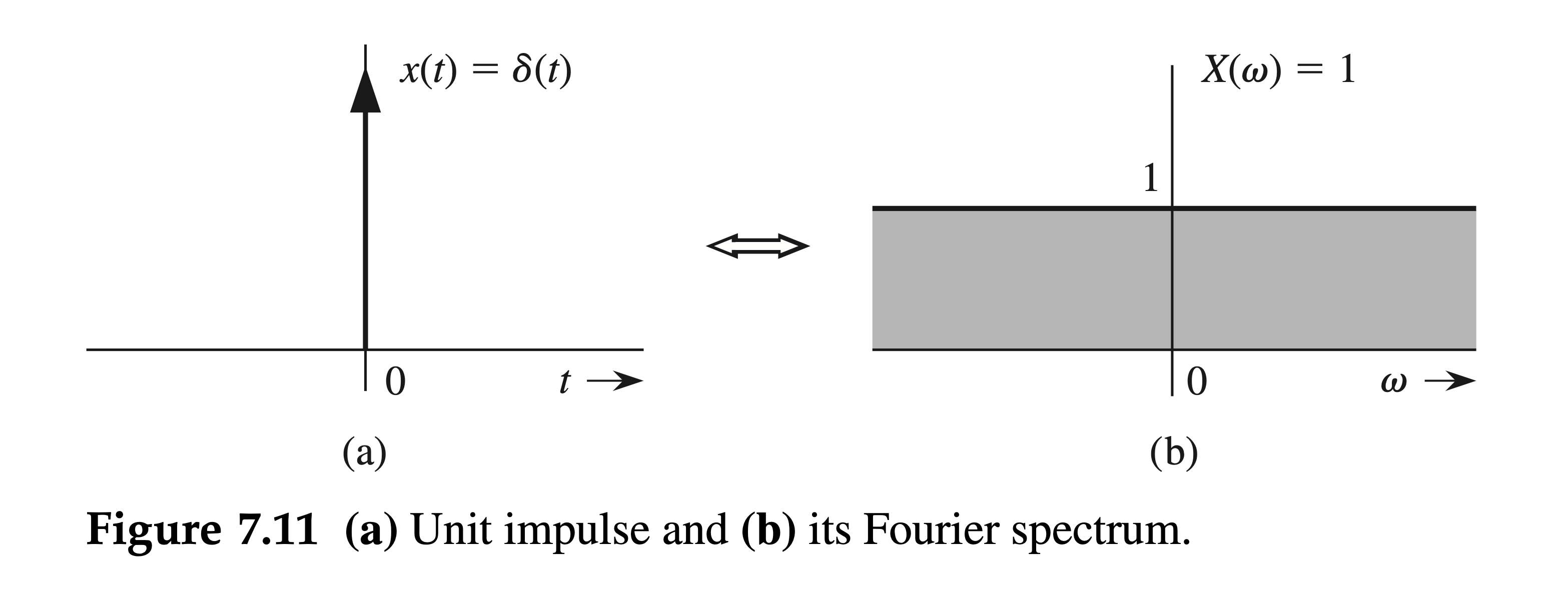
Using the sampling property of the impulse, we obtain $$\mathcal{F}[\delta (t)]={\int }_{-\mathrm{\infty }}^{\mathrm{\infty }}\delta (t)e^{-j\omega t}dt=1\text{ and }\delta (t)⟺1$$

Inverse Fourier Transform of the Dirac Delta Function

Figure 7.12

Find the inverse Fourier transform of $\delta (\omega )$.

---

On the basis of Eq. (7.10) and the sampling property of the impulse function, $${\mathcal{F}}^{-1}[\delta (\omega )]=\frac{1}{2\pi }{\int }_{-\mathrm{\infty }}^{\mathrm{\infty }}\delta (\omega )e^{j\omega t}d\omega =\frac{1}{2\pi }$$

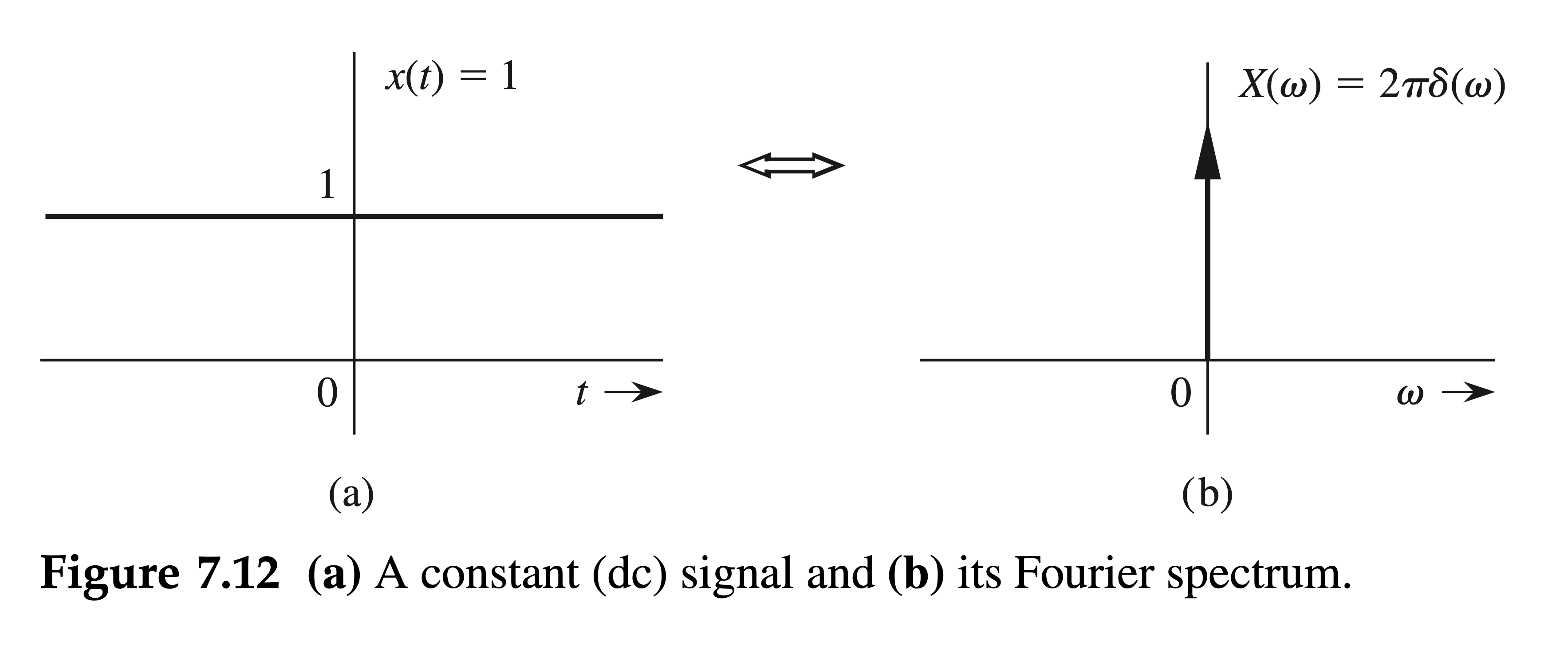
Therefore, $$\frac{1}{2\pi }⟺\delta (\omega )\text{ and }1⟺2\pi \delta (\omega )$$

This result shows that the spectrum of a constant signal $x(t)=1$ is an impulse $2\pi \delta (\omega )$, as illustrated in Fig. 7.12.

The result [Eq. (7.20)] could have been anticipated on qualitative grounds. Recall that the Fourier transform of $x(t)$ is a spectral representation of $x(t)$ in terms of everlasting exponential components of the form $e^{j\omega t}$. Now, to represent a constant signal $x(t)=1$, we need a single everlasting exponential $e^{j\omega t}$ with $\omega =0{.}^{†}$ This results in a spectrum at a single frequency $\omega =0$. Another way of looking at the situation is that $x(t)=1$ is a dc signal that has a single frequency $\omega =0$ (dc).

Inverse Fourier Transform of a Shifted Dirac Delta Function

Find the inverse Fourier transform of $\delta (\omega -{\omega }_0)$.

---

Using the sampling property of the impulse function, we obtain $${\mathcal{F}}^{-1}\left[\delta (\omega -{\omega }_0)\right]=\frac{1}{2\pi }{\int }_{-\mathrm{\infty }}^{\mathrm{\infty }}\delta (\omega -{\omega }_0)e^{j\omega t}d\omega =\frac{1}{2\pi }{e}^{j{\omega }_{0}t}$$

Therefore, $$\frac{1}{2\pi }{e}^{j{\omega }_{0}t}⟺\delta (\omega -{\omega }_0)\text{ and }{e}^{j{\omega }_{0}t}⟺2\pi \delta (\omega -{\omega }_0)$$

This result shows that the spectrum of an everlasting exponential $e^{j{\omega }_{0}t}$ is a single impulse at $\omega ={\omega }_0$. We reach the same conclusion by qualitative reasoning. To represent the everlasting exponential $e^{j{\omega }_{0}t}$, we need a single everlasting exponential $e^{j\omega t}$ with $\omega ={\omega }_0$. Therefore, the spectrum consists of a single component at frequency $\omega ={\omega }_0$. From Eq. (7.21) it follows that $$e^{-j{\omega }_{0}t}⟺2\pi \delta (\omega +{\omega }_0)$$

Fourier Transform of a Sinusoid

Figure 7.13

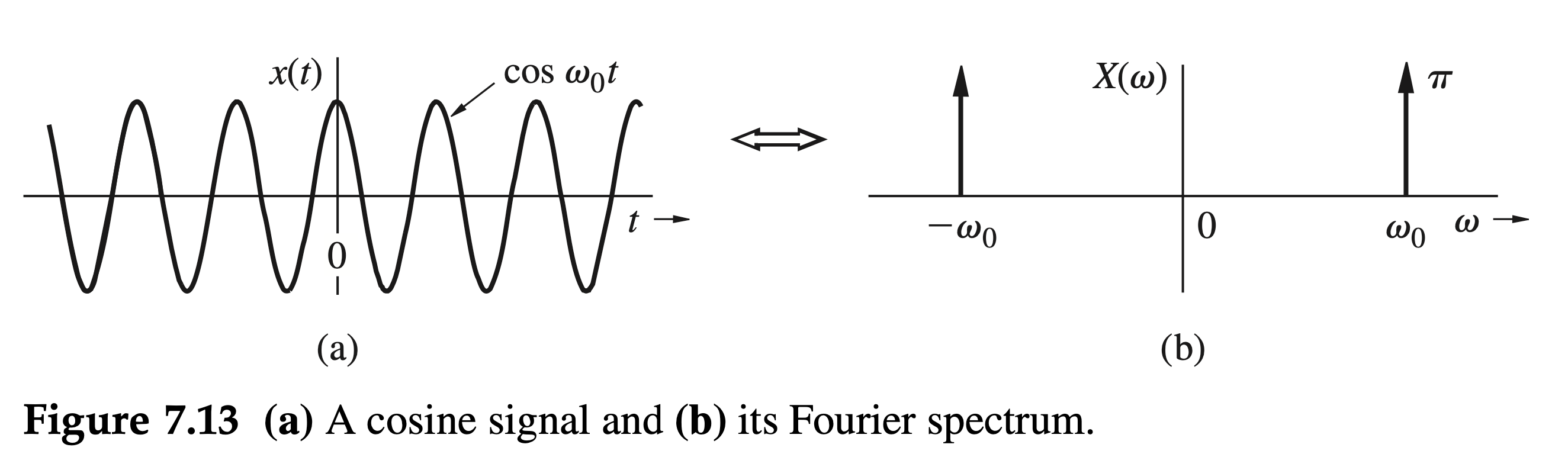
Find the Fourier transform of the everlasting sinusoid $\cos {\omega }_{0}t$ (Fig. 7.13a). ***

Recall Euler's formula $$\cos {\omega }_{0}t=\frac{1}{2}(e^{j{\omega }_{0}t}+e^{-j{\omega }_{0}t})$$

Applying Eq. (7.21), we obtain $$\cos {\omega }_{0}t⟺\pi [\delta (\omega +{\omega }_0)+\delta (\omega -{\omega }_0)]$$

The spectrum of $\cos {\omega }_{0}t$ consists of two impulses at ${\omega }_0$ and $-{\omega }_0$, as shown in Fig. 7.13b. The result also follows from qualitative reasoning. An everlasting sinusoid $\cos {\omega }_{0}t$ can be synthesized by two everlasting exponentials, $e^{j{\omega }_{0}t}$ and $e^{-j{\omega }_{0}t}$. Therefore, the Fourier spectrum consists of only two components of frequencies ${\omega }_0$ and $-{\omega }_0$.

Fourier Transform of a Periodic Signal

Determine the Fourier transform of a periodic signal $x(t)$ using its Fourier series representation. ***

We can use a Fourier series to express a periodic signal as a sum of exponentials of the form $e^{jn{\omega }_{0}t}$, whose Fourier transform is found in Eq. (7.21). Hence, we can readily find the Fourier transform of a periodic signal by using the linearity property in Eq. (7.15).

The Fourier series of a periodic signal $x(t)$ with period $T_0$ is given by $$x(t)=\sum _{n=-\mathrm{\infty }}^{\mathrm{\infty }}{D}_n{e}^{jn{\omega }_{0}t}{\omega }_0=\frac{2\pi }{T_0}$$

Taking the Fourier transform of both sides, we obtain ${}^{†}$ $$X(\omega )=2\pi \sum _{n=-\mathrm{\infty }}^{\mathrm{\infty }}{D}_n\delta (\omega -n{\omega }_0)$$

Fourier Transform of a Dirac Delta Train

Figure 7.14

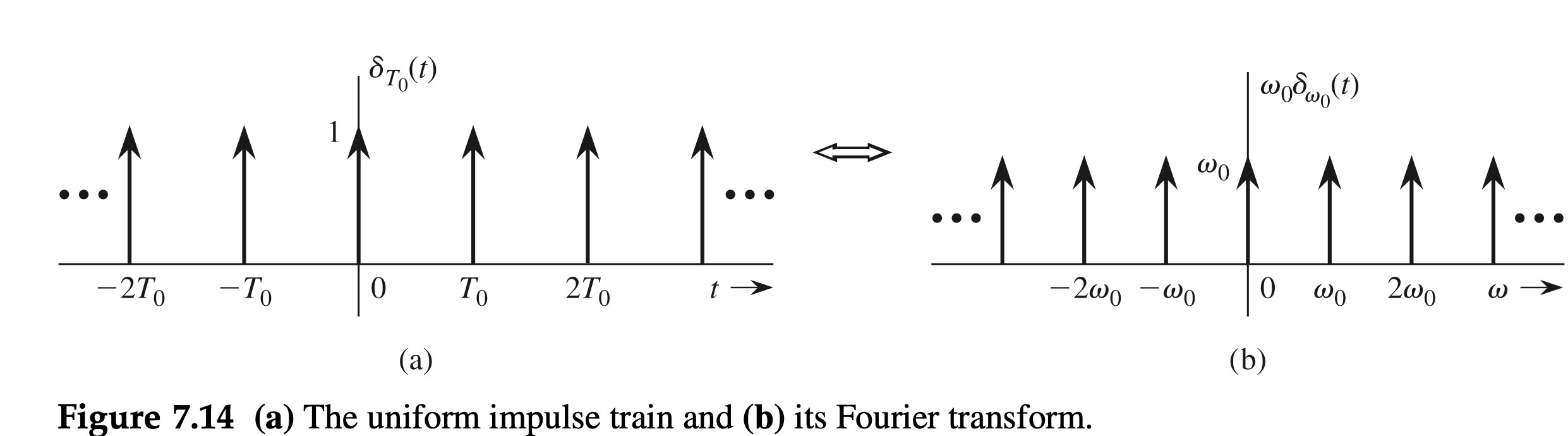
Determine the Fourier transform of a Dirac delta train ${\delta }_{T_0}(t)$ (Fig. 7.14a) using its Fourier series representation.

---

As shown in Eq. (6.24) from Ex. 6.9, the Fourier coefficients $D_n$ for ${\delta }_{T_0}(t)$ are constant $D_n=1/T_0$. From Eq. (7.22), the Fourier transform of ${\delta }_{T_0}(t)$ is therefore $$X(\omega )=\frac{2\pi }{T_0}\sum _{n=-\mathrm{\infty }}^{\mathrm{\infty }}\delta (\omega -n{\omega }_0)={\omega }_0{\delta }_{{\omega }_0}(\omega ),\text{ where }{\omega }_0=\frac{2\pi }{T_0}$$

The corresponding spectrum is shown in Fig. 7.14b.

Fourier Transform of the Unit Step Function

Figure 7.15

Find the Fourier transform of the unit step function $u(t)$.

---

Trying to find the Fourier transform of $u(t)$ by direct integration leads to an indeterminate result because $$U(\omega )={\int }_{-\mathrm{\infty }}^{\mathrm{\infty }}u(t)e^{-j\omega t}dt={\int }_0^{\mathrm{\infty }}{e}^{-j\omega t}dt={\frac{-1}{j\omega }{e}^{-j\omega t}|}_0^{\mathrm{\infty }}$$

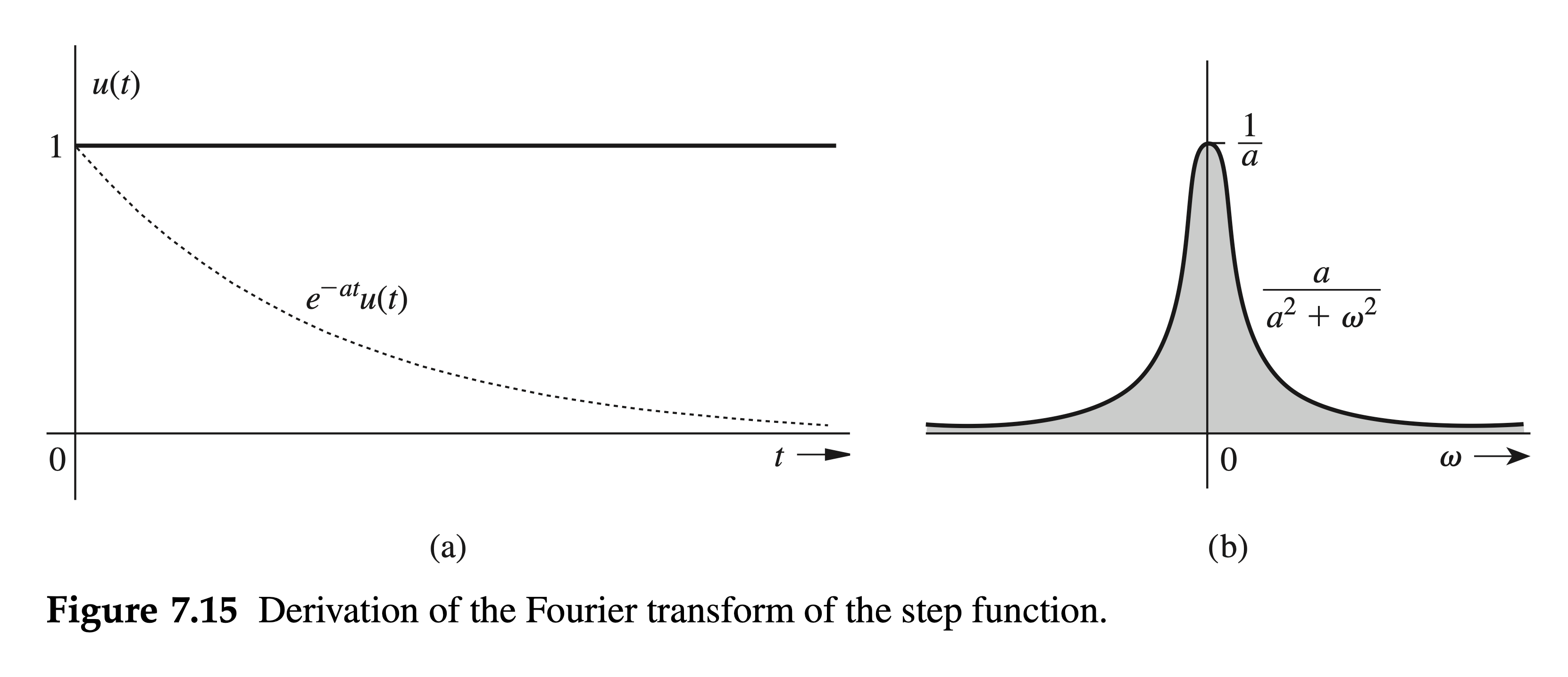
The upper limit of $e^{-j\omega t}$ as $t\to \mathrm{\infty }$ yields an indeterminate answer. So we approach this problem by considering $u(t)$ to be a decaying exponential $e^{-at}u(t)$ in the limit as $a\to 0$ (Fig. 7.15a). Thus, $$u(t)=\underset{a\to 0}{lim}{e}^{-at}u(t)$$ and $$U(\omega )=\underset{a\to 0}{lim}\mathcal{F}\{e^{-at}u(t)\}=\underset{a\to 0}{lim}\frac{1}{a+j\omega }$$

Expressing the right-hand side in terms of its real and imaginary parts yields $$U(\omega )=\underset{a\to 0}{lim}[\frac{a}{a^2+{\omega }^2}-j\frac{\omega }{a^2+{\omega }^2}]=\underset{a\to 0}{lim}\left[\frac{a}{a^2+{\omega }^2}\right]+\frac{1}{j\omega }$$

The function $a/(a^2+{\omega }^2)$ has interesting properties. First, the area under this function (Fig. 7.15b) is $\pi$ regardless of the value of $a$ : $${\int }_{-\mathrm{\infty }}^{\mathrm{\infty }}\frac{a}{a^2+{\omega }^2}d\omega ={{\tan }^{-1}\frac{\omega }{a}|}_{-\mathrm{\infty }}^{\mathrm{\infty }}=\pi$$

Second, when $a\to 0$, this function approaches zero for all $\omega \ne 0$, and all its area ( $\pi$ ) is concentrated at a single point $\omega =0$. Clearly, as $a\to 0$, this function approaches an impulse of strength $\pi$. Thus, $$U(\omega )=\pi \delta (\omega )+\frac{1}{j\omega }$$

Note that $u(t)$ is not a "true" dc signal because it is not constant over the interval $-\mathrm{\infty }$ to $\mathrm{\infty }$. To synthesize "true" dc, we require only one everlasting exponential with $\omega =0$ (impulse at $\omega =0$ ). The signal $u(t)$ has a jump discontinuity at $t=0$. It is impossible to synthesize such a signal with a single everlasting exponential $e^{j\omega t}$. To synthesize this signal from everlasting exponentials, we need, in addition to an impulse at $\omega =0$, all the frequency components, as indicated by the term $1/j\omega$ in Eq. (7.23).

Fourier Transform of the Sign Function

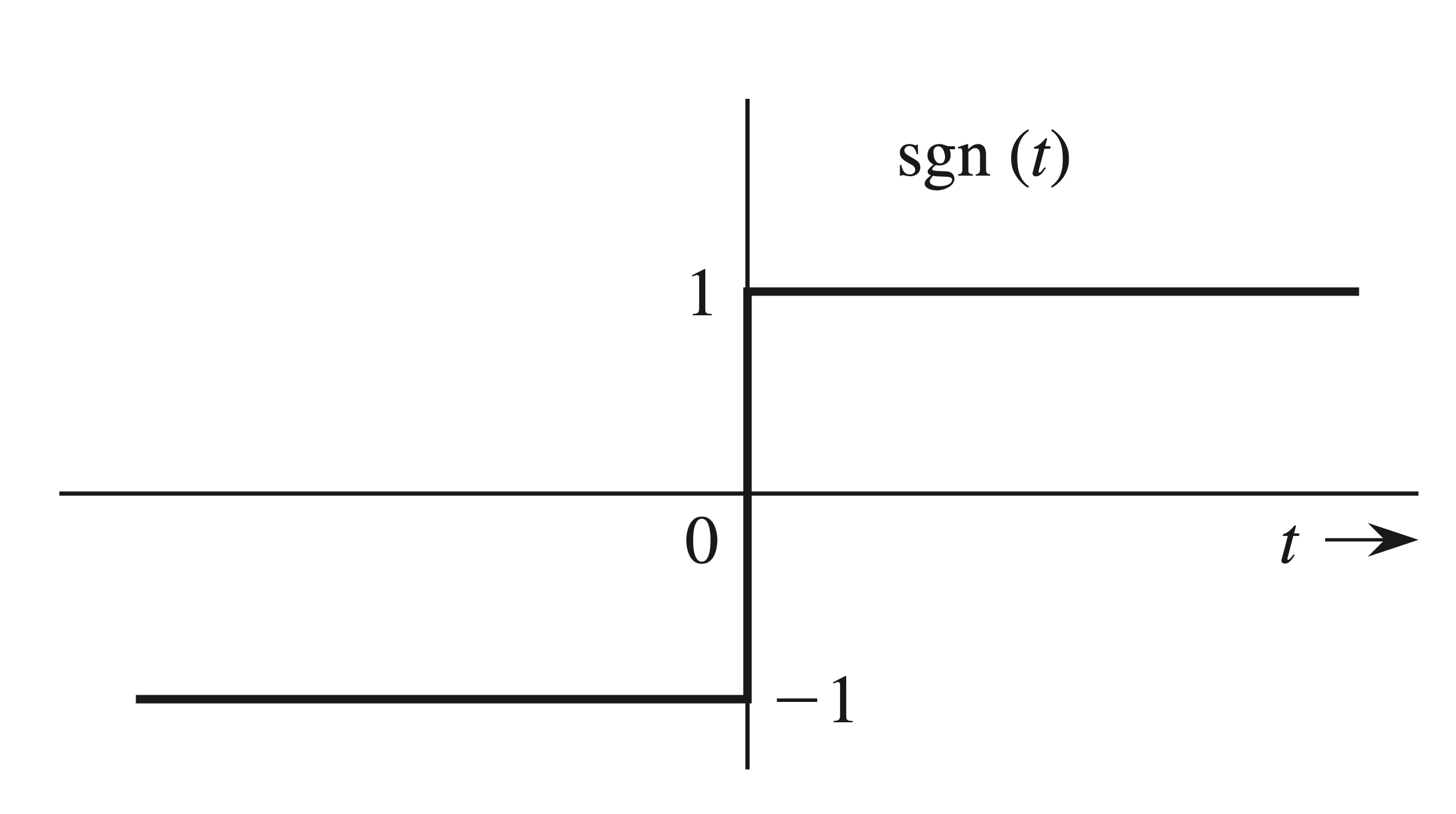
Find the Fourier transform of the sign function $\mathrm{sgn}(t)$ [pronounced signum $(t)$ ], depicted in Fig. 7.16. ***

Observe that $$\mathrm{sgn}(t)+1=2u(t)⟹\mathrm{sgn}(t)=2u(t)-1$$

Using Eqs. (7.20) and (7.23) and the linearity property, we obtain $$\mathrm{sgn}(t)⟺\frac{2}{j\omega }$$

---

1. At $|x|=0.5$, we require rect $(x)=0.5$ because the inverse Fourier transform of a discontinuous signal converges to the mean of its two values at the discontinuity.↩︎