System Stability
Sources:
- B. P. Lathi & Roger Green. (2021). Chapter 2: Time-Domain Analysis of Continuous-Time Systems. Signal Processing and Linear Systems (2nd ed., pp. 168-195). Oxford University Press.
Stability is an important system property. Two types of system stability are generally considered: external (BIBO) stability and internal (asymptotic) stability. Let us consider both stability types in turn.
Types of equilibrium
If, in the absence of an external input, a system remains in a particular state (or condition) indefinitely, then that state is said to be an equilibrium state of the system.
Take a right circular cone as example. Such a cone can be made to stand forever on its circular base, on its apex, or on its side. For this reason, these three states of the cone are said to be equilibrium states. Qualitatively, however, the three states show very different behavior.
- If the cone, standing on its circular base, were to be disturbed slightly and then left to itself, it would eventually return to its original equilibrium position. In such a case, the cone is said to be in stable equilibrium.
- In contrast, if the cone stands on its apex, then the slightest disturbance will cause the cone to move farther and farther away from its equilibrium state. The cone in this case is said to be in an unstable equilibrium.
- The cone lying on its side, if disturbed, will neither go back to the original state nor continue to move farther away from the original state. Thus, it is said to be in a neutral equilibrium.
Clearly, when a system is in stable equilibrium, application of a small disturbance (input) produces a small response.
In contrast, when the system is in unstable equilibrium, even a minuscule disturbance (input) produces an unbounded response. The BIBO-stability definition can be understood in the light of this concept.
External (BIBO) stability
If every bounded input produces bounded output, the system is (BIBO) stable. In contrast, if even one bounded input results in unbounded response, the system is (BIBO) unstable.
Recall from the past post, for a LTI system, \[ y(t)=h(t) * x(t)=\int_{-\infty}^{\infty} h(\tau) x(t-\tau) d \tau \]
Therefore, \[ |y(t)| \leq \int_{-\infty}^{\infty}|h(\tau)||x(t-\tau)| d \tau \]
Moreover, if \(x(t)\) is bounded, then \(|x(t-\tau)|<K_1<\infty\), and \[ |y(t)| \leq K_1 \int_{-\infty}^{\infty}|h(\tau)| d \tau \]
Hence for BIBO stability, \[ \int_{-\infty}^{\infty}|h(\tau)| d \tau<\infty \]
This is a sufficient condition for BIBO stability. We can show that this is also a necessary condition (see Prob. 2.5-7).
Therefore, for an LTIC system, if its impulse response \(h(t)\) is absolutely integrable, the system is (BIBO) stable. Otherwise, it is (BIBO) unstable.
In addition, we shall show in Ch. 6 that a necessary (but not sufficient) condition for an LTIC system described by Eq. (2.1) to be BIBO-stable is \(M \leq N\). If \(M>N\), the system is unstable. This is one of the reasons to avoid systems with \(M>N\).
External (BIBO) stability may not be a correct indication of internal stability. Indeed, some systems that appear stable by the BIBO criterion may be internally unstable. This is like a room on fire inside a house: no trace of fire is visible from outside, but the entire house will be burned to ashes.
Examples
Determine whether the following systems are BIBO-stable:
\(y(t)=x^2(t)\),
\(y(t)=t x(t)\), and
\(y(t)=\frac{d}{d t} x(t)\)
- This system squares an input to produce the output. If the input is bounded, which is to say that \(|x(t)| \leq M_x<\infty\) for all \(t\), then we see that \[ |y(t)|=\left|x^2(t)\right|=|x(t)|^2 \leq M_x^2<\infty \]
Since the output amplitude is guaranteed to be bounded for any bounded-amplitude input, the system \(y(t)=x^2(t)\) is BIBO-stable.
We can prove that \(y(t)=t x(t)\) is not BIBO-stable with a simple example. The bounded-amplitude input \(x(t)=u(t)\) produces the output \(y(t)=t u(t)\) whose amplitude grows to infinity as \(t \rightarrow \infty\). Thus, \(y(t)=t x(t)\) is a BIBO-unstable system.
We can prove that \(y(t)=\frac{d}{d t} x(t)\) is not BIBO-stable with an example. The bounded-amplitude input \(x(t)=u(t)\) produces the output \(y(t)=\delta(t)\) whose amplitude is infinite at \(t=0\). Thus, \(y(t)=\frac{d}{d t} x(t)\) is a BIBO-unstable system.
Internal (Asymptotic) stability
For an LTI system, zero state, in which all initial conditions are zero, is an equilibrium state.
Now suppose an LTI system is in zero state and we change this state by creating small nonzero initial conditions (a small disturbance). These initial conditions will generate signals consisting of characteristic modes in the system.
By analogy with the cone, if the system is stable, it should eventually return to zero state. In other words, when left to itself, every mode in a stable system arising as a result of nonzero initial conditions should approach 0 as \(t \rightarrow \infty\).
However, if even one of the modes grows with time, the system will never return to zero state, and the system would be identified as unstable.
In the borderline case, some modes neither decay to zero nor grow indefinitely, while all the remaining modes decay to zero. This case is like the neutral equilibrium in the cone. Such a system is said to be marginally stable.
Internal stability is also called asymptotic stability or stability in the sense of Lyapunov.
For a system characterized by1 \[ \begin{aligned} & \frac{d^N y(t)}{d t^N}+a_1 \frac{d^{N-1} y(t)}{d t^{N-1}}+\cdots+a_{N-1} \frac{d y(t)}{d t}+a_N y(t) \\ & \quad=b_{N-M} \frac{d^M x(t)}{d t^M}+b_{N-M+1} \frac{d^{M-1} x(t)}{d t^{M-1}}+\cdots+b_{N-1} \frac{d x(t)}{d t}+b_N x(t) , \end{aligned} \] we can restate the internal stability criterion in terms of the location of the \(N\) characteristic roots \[ \lambda_1, \lambda_2, \ldots, \lambda_N \] of the system in a complex plane. The characteristic modes are of the form \(e^{\lambda_k t}\) or \(t^r e^{\lambda_k t}\). The locations of various roots in the complex plane and the corresponding modes are shown in Fig. 2.17.

These modes \(\rightarrow 0\) as \(t \rightarrow \infty\) if \(\operatorname{Re}\) \(\lambda_k<0\). In contrast, the modes \(\rightarrow \infty\) as \(t \rightarrow \infty\) if \(\operatorname{Re} \lambda_k>0\). \(^{+}\)
From Fig. 2.17, we see that a system is (asymptotically) stable if all its characteristic roots lie in the LHP, that is, if \(\operatorname{Re} \lambda_k<0\) for all \(k\).
If even a single characteristic root lies in the RHP, the system is (asymptotically) unstable.
Modes due to roots on the imaginary axis \(\left(\lambda= \pm j \omega_0\right)\) are of the form \(e^{ \pm j \omega_0 t}\). Hence, if some roots are on the imaginary axis, and all the remaining roots are in the LHP, the system is marginally stable (assuming that the roots on the imaginary axis are not repeated) (Basically, marginally stable means stable for real roots).
If the imaginary axis roots are repeated, the characteristic modes are of the form \(t^r e^{ \pm j \omega_k{ }^2}\), which do grow with time indefinitely. Hence, the system is unstable. Figure 2.18 shows stability regions in the complex plane.
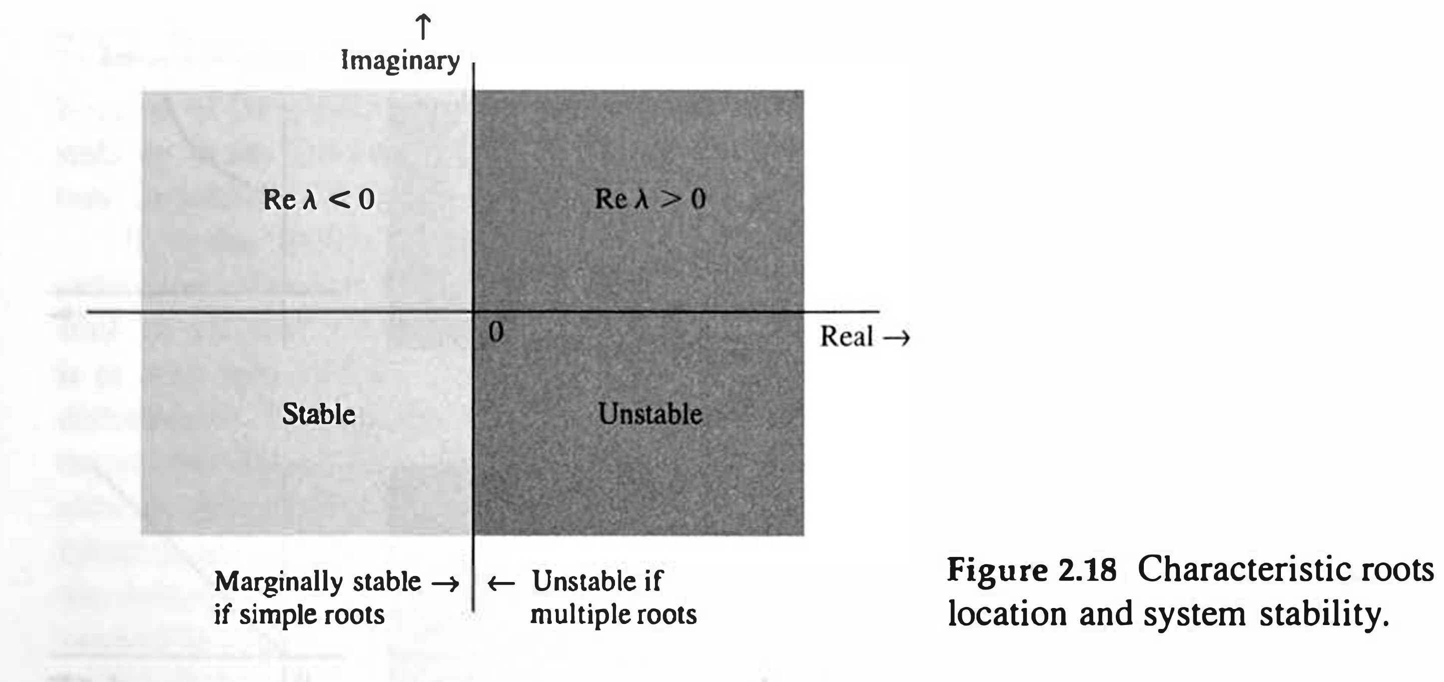
To summarize: 1. An LTIC system is (asymptotically) stable if, and only if, all the characteristic roots are in the LHP. The roots may be simple (unrepeated) or repeated. 2. An LTIC system is unstable if, and only if, one or both of the following conditions exist: (i) at least one root is in the RHP; (ii) there are repeated roots on the imaginary axis. 3. An LTIC system is marginally stable if, and only if, there are no roots in the RHP, and there are some unrepeated roots on the imaginary axis.
Note: for the root at the origin, it's seen as on the imaginary axis.
Relationship between BIBO and asymptotic stability
External stability is determined by applying an external input with zero initial conditions, while internal stability is determined by applying the nonzero initial conditions and no external input. This is why these stabilities are also called the zero-state stability and the zero-input stability, respectively.
# TODO: Can't understand why BIBO is related to zero-state condition.
The internal stability is determined by applying the nonzero initial conditions and no external input. So it is related to the zero-input response.↩︎