Sources:

1. B. P. Lathi & Roger Green. (2021). Chapter 2: Time-Domain Analysis of Continuous-Time Systems. Signal Processing and Linear Systems (2nd ed., pp. 168-195). Oxford University Press.

This section is devoted to the determination of the zero-state response(see past post) of an LTIC system. We shall assume that the systems discussed in this section are in the zero state unless mentioned otherwise.

The zero-state response

We shall use the superposition property for finding the system response to an arbitrary input $x(t)$.

Fig. 2.3a-2.3b

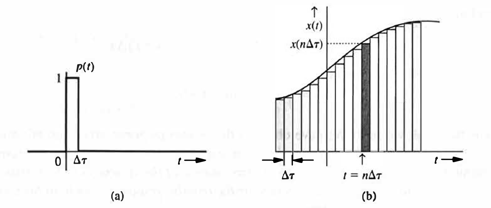
Let us define a basic pulse $p(t)$ of unit height and width $\mathrm{\Delta }\tau$, starting at $t=0$ as illustrated in Fig. 2.3a. Figure 2.3b shows an input $x(t)$ as a sum of narrow rectangular pulses. The pulse starting at $t=n\mathrm{\Delta }\tau$ in Fig. 2.3b has a height $x(n\mathrm{\Delta }\tau )$ and can be expressed as $x(n\mathrm{\Delta }\tau )p(t-n\mathrm{\Delta }\tau )$. Now, $x(t)$ is the sum of all such pulses. Hence, $$x(t)=\underset{\mathrm{\Delta }\tau \to 0}{lim}\sum _{\tau }x(n\mathrm{\Delta }\tau )p(t-n\mathrm{\Delta }\tau )=\underset{\mathrm{\Delta }\tau \to 0}{lim}\sum _{\tau }\left[\frac{x(n\mathrm{\Delta }\tau )}{\mathrm{\Delta }\tau }\right]p(t-n\mathrm{\Delta }\tau )\mathrm{\Delta }\tau .$$

The term $[\frac{x(n\mathrm{\Delta }\tau )}{\mathrm{\Delta }\tau }]p(t-n\mathrm{\Delta }\tau )$ represents a pulse $p(t-n\mathrm{\Delta }\tau )$ with height $[x(n\mathrm{\Delta }\tau )/\mathrm{\Delta }\tau ]$. As $\mathrm{\Delta }\tau \to 0$, the height of this strip $\to \mathrm{\infty }$, but its area remains $x(n\mathrm{\Delta }\tau )$. Hence, this strip approaches an impulse $x(n\mathrm{\Delta }\tau )\delta (t-n\mathrm{\Delta }\tau )$ as $\mathrm{\Delta }\tau \to 0$ (Fig. 2.3e)¹.

Fig. 2.3e

Therefore, $$x(t)=\underset{\mathrm{\Delta }\tau \to 0}{lim}\sum _{\tau }x(n\mathrm{\Delta }\tau )\delta (t-n\mathrm{\Delta }\tau )\mathrm{\Delta }\tau .$$

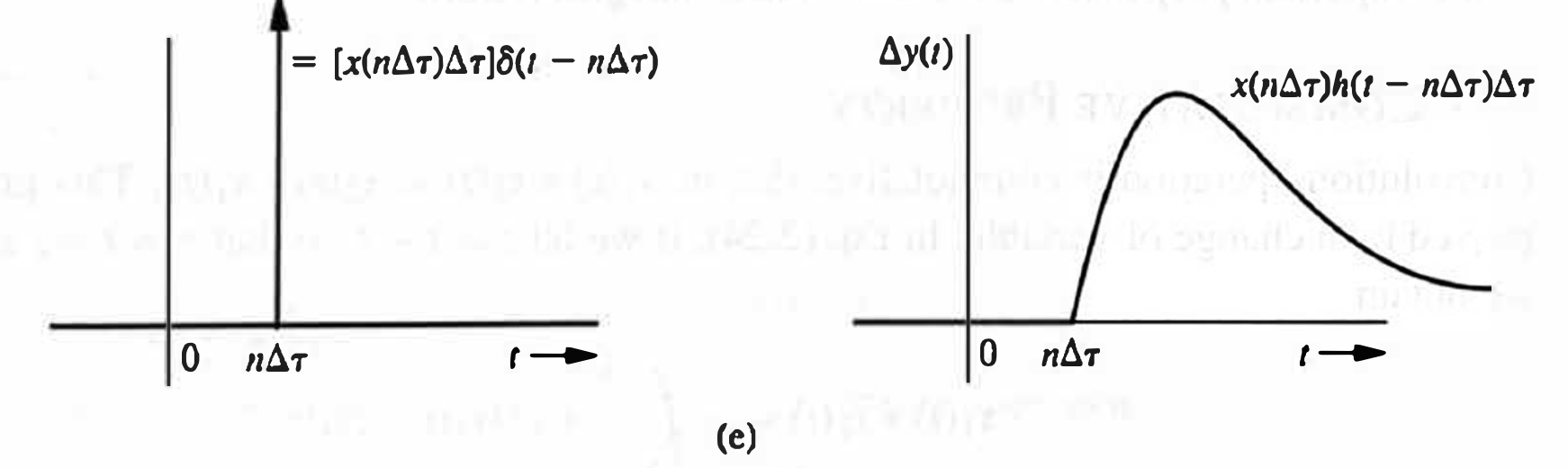
To find the response for this input $x(t)$, we consider the input and the corresponding output pairs, as shown in Figs. 2.3c-2.3e

Figs. 2.3c-2.3e

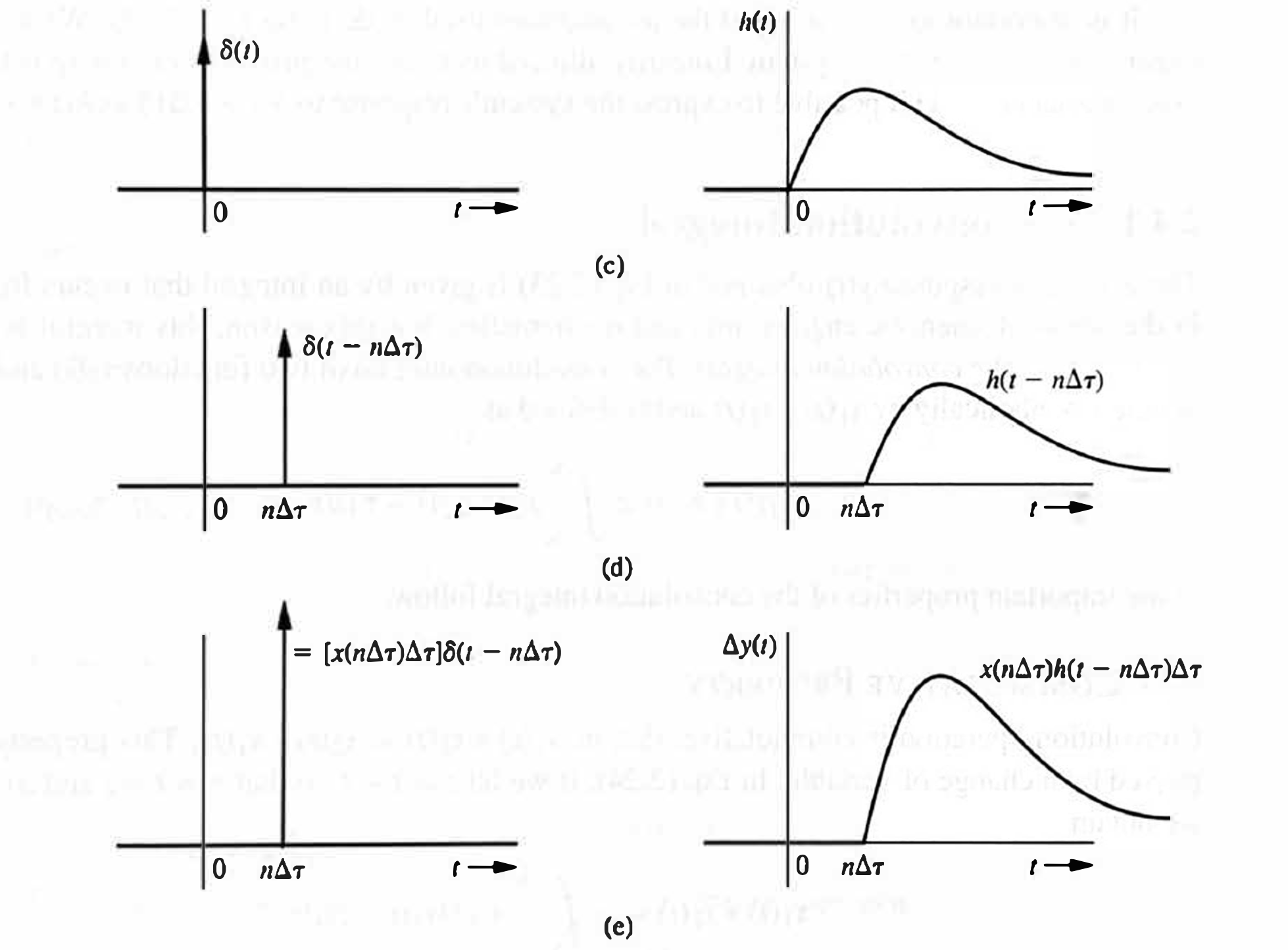
and also shown by directed arrow notation as follows: $$\begin{array}{rl}\text{ input }& ⟹\text{ output }\\ \delta (t)& ⟹h(t)\\ \delta (t-n\mathrm{\Delta }\tau )& ⟹h(t-n\mathrm{\Delta }\tau )\\ [x(n\mathrm{\Delta }\tau )\mathrm{\Delta }\tau ]\delta (t-n\mathrm{\Delta }\tau )& ⟹[x(n\mathrm{\Delta }\tau )\mathrm{\Delta }\tau ]h(t-n\mathrm{\Delta }\tau )\\ \underset{x(t)\text{ [see Eq. (2.22)] }}{\underbrace{\underset{\mathrm{\Delta }\tau \to 0}{lim}\sum _{\tau }x(n\mathrm{\Delta }\tau )\delta (t-n\mathrm{\Delta }\tau )\mathrm{\Delta }\tau }}& ⟹\underset{y(t)}{\underbrace{\underset{\mathrm{\Delta }\tau 0}{lim}\sum _{\tau }x(n\mathrm{\Delta }\tau )h(t-n\mathrm{\Delta }\tau )\mathrm{\Delta }\tau }}\end{array}$$

Therefore, in a linear time-invariant (LTI) system, $$\begin{array}{rl}& y(t)\\ & =\underset{\mathrm{\Delta }\tau \to 0}{lim}\sum _{\tau }x(n\mathrm{\Delta }\tau )h(t-n\mathrm{\Delta }\tau )\mathrm{\Delta }\tau \\ \text{(1)}& & ={\int }_{-\mathrm{\infty }}^{\mathrm{\infty }}x(\tau )h(t-\tau )d\tau \end{array}$$

Thus, we have obtained that, in a LTI system (also, recall that we have a zero-state assumption), knowing the unit impulse response $h(t)$, we can determine the response $y(t)$ to an arbitrary input $x(t)$.

The LTI system assumtption is important. Linearity allowed us to use the principle of superposition, and time invariance made it possible to express the system's response to $\delta (t-n\mathrm{\Delta }\tau )$ as $h(t-n\mathrm{\Delta }\tau )$.

If the system is time-varying, then the system response to the input $\delta (t-n\mathrm{\Delta }\tau )$ cannot be expressed as $h(t-n\mathrm{\Delta }\tau )$ but instead has the form $h(t,n\mathrm{\Delta }\tau )$. Use of this form modifies $\text{(1)}$ to $$y(t)={\int }_{-\mathrm{\infty }}^{\mathrm{\infty }}x(\tau )h(t,\tau )d\tau$$

where $h(t,\tau )$ is the system response at instant $t$ to a unit impulse input located at $\tau$.

The Convolution Integral

The zero-state response $y(t)$ obtained in $\text{(1)}$ is given by an integral which is given a special name: the convolution integral.

The convolution integral of two functions $x_1(t)$ and $x_2(t)$ is denoted symbolically by $x_1(t)\ast x_2(t)$ and is defined as $$\begin{array}{}\text{(2)}& & x_1(t)\ast x_2(t)\text{(3)}& & \triangleq {\int }_{-\mathrm{\infty }}^{+\mathrm{\infty }}{x}_1(\tau )x_2(t-\tau )d\tau .\end{array}$$

It can be proved easily that convolution is a linear operation.

Properties of the convolution integral

Some important properties of the convolution integral follow.

The Commutative Property

Convolution operation is commutative; that is, $x_1(t)\ast x_2(t)=x_2(t)\ast x_1(t)$. This property can be proved by a change of variable. In $\text{(3)}$, if we let $z=t-\tau$ so that $\tau =t-z$ and $d\tau =-dz$, we obtain $$\begin{array}{rl}{x}_1(t)\ast x_2(t)& =-{\int }_{\mathrm{\infty }}^{-\mathrm{\infty }}{x}_2(z)x_1(t-z)dz\\ & ={\int }_{-\mathrm{\infty }}^{\mathrm{\infty }}{x}_2(z)x_1(t-z)dz\\ & =x_2(t)\ast x_1(t)\end{array}$$

The Distributive Property

According to the distributive property, $$x_1(t)\ast [x_2(t)+x_3(t)]=x_1(t)\ast x_2(t)+x_1(t)\ast x_3(t)$$

The Associative Property

According to the associative property, $$x_1(t)\ast [x_2(t)\ast x_3(t)]=[x_1(t)\ast x_2(t)]\ast x_3(t)$$

The proofs of the distributive property and the Associative Property follow directly from the definition of the convolution integral.

The Shift Property

If $$x_1(t)\ast x_2(t)=c(t)$$ then $$x_1(t)\ast x_2(t-T)=x_1(t-T)\ast x_2(t)=c(t-T)$$

More generally, we see that $$x_1(t-T_1)\ast x_2(t-T_2)=c(t-T_1-T_2).$$

Proof: We are given $$x_1(t)\ast x_2(t)={\int }_{-\mathrm{\infty }}^{\mathrm{\infty }}{x}_1(\tau )x_2(t-\tau )d\tau =c(t)$$

Therefore, $$\begin{array}{rl}{x}_1(t)\ast x_2(t-T)& ={\int }_{-\mathrm{\infty }}^{\mathrm{\infty }}{x}_1(\tau )x_2(t-T-\tau )d\tau \\ & =c(t-T).\end{array}$$

Convolution with a Unit Impulse

Convolution of a function $x(t)$ with a unit impulse $\delta (t)$ results in the function $x(t)$ itself. By definition of convolution, $$x(t)\ast \delta (t)={\int }_{-\mathrm{\infty }}^{+\mathrm{\infty }}x(\tau )\delta (t-\tau )d\tau$$

Because $\delta (t-\tau )$ is an impulse located at $\tau =t$, according to the sampling property of the impulse (see before post, the integral here is just the value of $x(\tau )$ at $\tau =t$, that is, $x(t)$. Therefore, $$x(t)\ast \delta (t)=x(t).$$

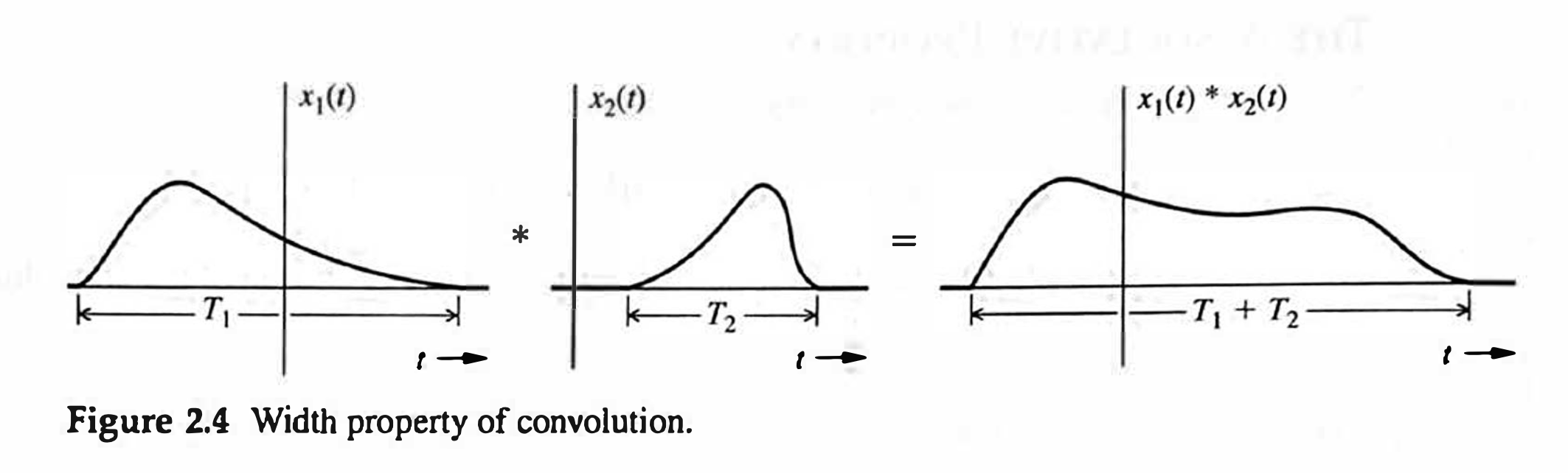
The Width Property

If the durations (widths) of $x_1(t)$ and $x_2(t)$ are finite, given by $T_1$ and $T_2$, respectively, then the duration (width) of $x_1(t)\ast x_2(t)$ is $T_1+T_2$ (Fig. 2.4). The proof of this property follows readily from the graphical considerations discussed later.

Fig. 2.4

The (zero-state) response and causility

For a LTIC system, since it has already been a LTI system, its (zero-state) response $y(t)$ is also $$\begin{array}{rl}& y(t)\\ & =x(t)\ast h(t)\\ \text{(4)}& & ={\int }_{-\mathrm{\infty }}^{\mathrm{\infty }}x(\tau )h(t-\tau )d\tau .\end{array}$$

The causality restriction on both signals and systems further simplifies the limits of integration in $\text{(4)}$. By definition, the response of a causal system cannot begin before its input begins. Consequently, the causal system's response to a unit impulse $\delta (t)$ (which is located at $t=0$ ) cannot begin before $t=0$. Therefore, a causal system's unit impulse response $h(t)$ is a causal signal.

Fig. 2.5

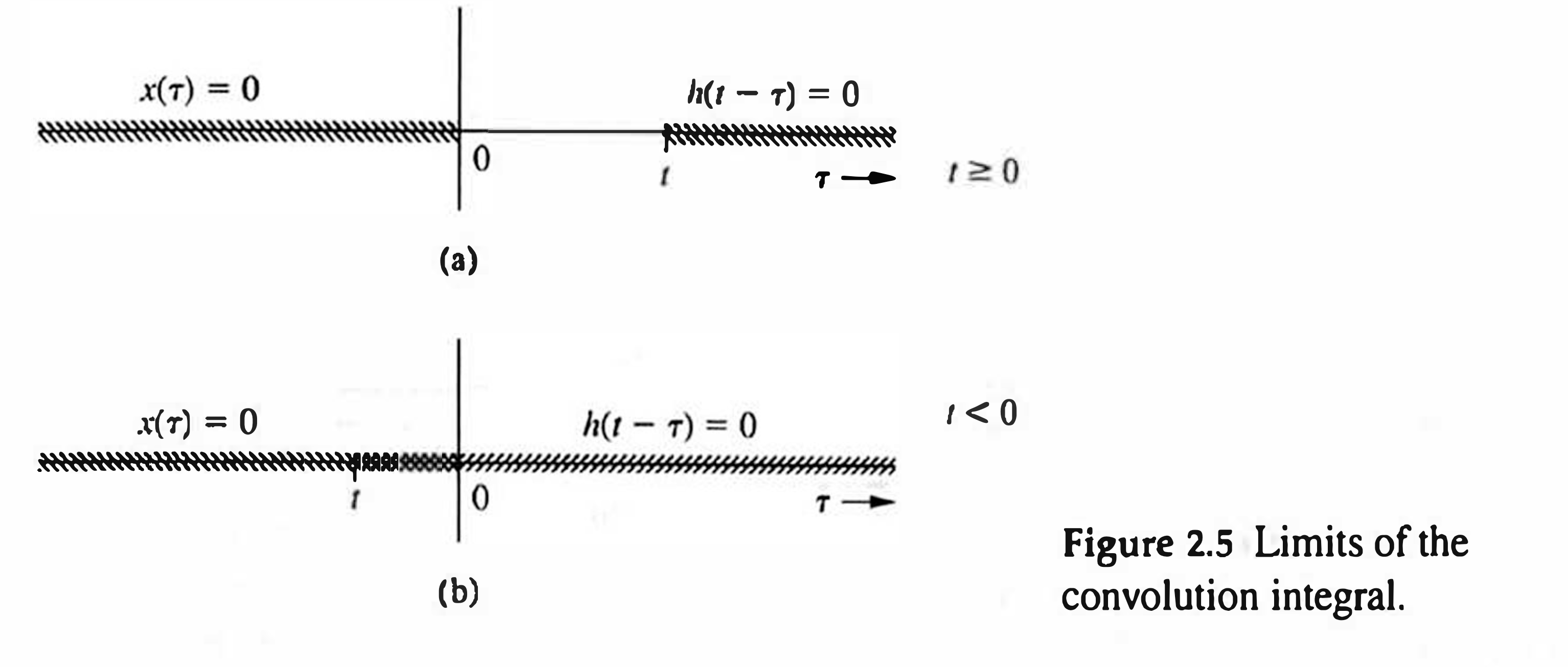
It is important to remember that the integration in $\text{(4)}$ is performed with respect to $\tau$ (not $t$ ). If the input $x(t)$ is causal, $x(\tau )=0$ for $\tau <0$. Therefore, $x(\tau )=0$ for $\tau <0$, as illustrated in Fig. 2.5a.

Similarly, if $h(t)$ is causal, $h(t-\tau )=0$ for $t-\tau <0$; that is, for $\tau >t$, as depicted in Fig. 2.5a. Therefore, the product $x(\tau )h(t-\tau )=0$ everywhere except over the nonshaded interval $0\le \tau \le t$ shown in Fig. 2.5a (assuming $t\ge 0$ ).

Observe that if $t$ is negative, $x(\tau )h(t-\tau )=0$ for all $\tau$, as shown in Fig. 2.5b.

Therefore, $\text{(4)}$ reduces to $$y(t)=x(t)\ast h(t)=\{\begin{array}{ll}{\int }_{0^{-}}^{t}x(\tau )h(t-\tau )d\tau & t\ge 0\\ 0& t<0\end{array}$$

The lower limit of integration is taken as $0^{-}$ to avoid the difficulty in integration that can arise if $x(t)$ contains an impulse at the origin. This result shows that if $x(t)$ and $h(t)$ are both causal, the response $y(t)$ is also causal.

Example: Computing the Zero-State Response

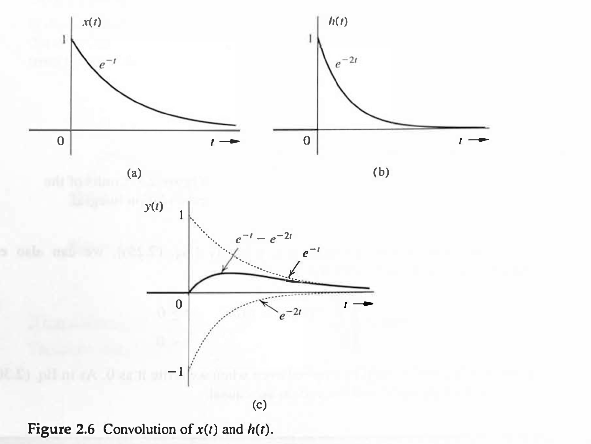
For an LTIC system with the unit impulse response $h(t)=e^{-2t}u(t)$, determine the response $y(t)$ for the input $$x(t)=e^{-t}u(t)$$

Solution:

Here, both $x(t)$ and $h(t)$ are causal (Fig. 2.6).

Fig. 2.6

Hence, we obtain $$y(t)={\int }_0^{t}x(\tau )h(t-\tau )d\tau t\ge 0$$

Because $x(t)=e^{-t}u(t)$ and $h(t)=e^{-2t}u(t)$, $$x(\tau )=e^{-\tau }u(\tau )\text{ and }h(t-\tau )=e^{-2(t-\tau )}u(t-\tau )$$

Remember that the integration is performed with respect to $\tau$ (not $t$ ), and the region of integration is $0\le \tau \le t$. Hence, $\tau \ge 0$ and $t-\tau \ge 0$. Therefore, $u(\tau )=1$ and $u(t-\tau )=1$; consequently, $$y(t)={\int }_0^t{e}^{-\tau }{e}^{-2(t-\tau )}d\tau t\ge 0$$ Because this integration is with respect to $\tau$, we can pull $e^{-2t}$ outside the integral, giving us $$y(t)=e^{-2t}{\int }_0^t{e}^{\tau }d\tau =e^{-2t}(e^t-1)=e^{-t}-e^{-2t}t\ge 0$$

Moreover, $y(t)=0$ when $t<0$ [see Eq. (2.30)]. Therefore, $$y(t)=(e^{-t}-e^{-2t})u(t)$$

The response is depicted in Fig. 2.6c.

Interconnected systems

image-20240509134923010

---

1. By its definition, the response of unit impulse $\delta (t)$ is denoted as $h(t)$, i.e., must be denotated with symbol $h$.↩︎