Deep Q Learning
Deep Q-learning or deep Q-network (DQN) is one of the earliest and most successful algorithms that introduce deep neural networks into RL.
DQN is not Q learning, at least not the specific Q learning algorithm introduced in my post, but it shares the core idea of Q learning.
Sources:
- Shiyu Zhao. Chapter 8: Value Function Approximation. Mathematical Foundations of Reinforcement Learning.
- DQN 2013 paper
- Reinforcement Learning Explained Visually (Part 5): Deep Q Networks, step-by-step by Ketan Doshi
- My github repo for DQN
Deep Q learning
Recalling that, we can use following update rule to do Q-learning with function approximation \[ w_{t+1}=w_t+\alpha_t\left[r_{t+1}+\gamma \color{orange}{\max _{a \in \mathcal{A}\left(s_{t+1}\right)} \hat{q}\left(s_{t+1}, a, w_t\right)}-\hat{q}\left(s_t, a_t, w_t\right)\right] \nabla_w \hat{q}\left(s_t, a_t, w_t\right) . \] However, this process is not so easy-to-implement with modern deep learning tools1. In contrast, deep Q-learning aims to minimize the loss function: \[ \color{purple}{J(w)=\mathbb{E}\left[\left(R+\gamma \max _{a \in \mathcal{A}\left(S^{\prime}\right)} \hat{q}\left(S^{\prime}, a, w\right)-\hat{q}(S, A, w)\right)^2\right]}, \] where \(\left(S, A, R, S^{\prime}\right)\) are random variables. - This is actually the Bellman optimality error. That is because \[ q(s, a)=\mathbb{E}\left[R_{t+1}+\gamma \max _{a \in \mathcal{A}\left(S_{t+1}\right)} q\left(S_{t+1}, a\right) \mid S_t=s, A_t=a\right], \quad \forall s, a \]
The value of \(R+\gamma \max _{a \in \mathcal{A}\left(S^{\prime}\right)} \hat{q}\left(S^{\prime}, a, w\right)-\hat{q}(S, A, w)\) should be zero in the expectation sense
Techniques
The target network
The gradient of the loss function is hard to compute since, in the equation, the parameter \(w\) not only appears in \(\hat{q}(S, A, w)\) but also in \[ y \doteq R+\gamma \max _{a \in \mathcal{A}\left(S^{\prime}\right)} \hat{q}\left(S^{\prime}, a, w\right) \] For the sake of simplicity, we assume that \(w\) in \(y\) is fixed (at least for a while) when we calculate the gradient.
NOTE: This assumtion looks not rigorous, in fact, I think it's an engineering choice and I don't have a mathmatical proof of the convergence of DQN under this assumption. There are some intuitive explanations for it, tough.
To do that, we introduce two networks. - One is a main network representing \(\hat{q}(s, a, w)\) - The other is a target network \(\hat{q}\left(s, a, w_T\right)\).
The loss function in this case degenerates to \[ J=\mathbb{E}\left[\left(R+\gamma \max _{a \in \mathcal{A}\left(S^{\prime}\right)} \color{red}{\hat{q}\left(S^{\prime}, a, w_T\right)}-\color{blue}{\hat{q}(S, A, w)}\right)^2\right] \] where \(w_T\) is the target network parameter.
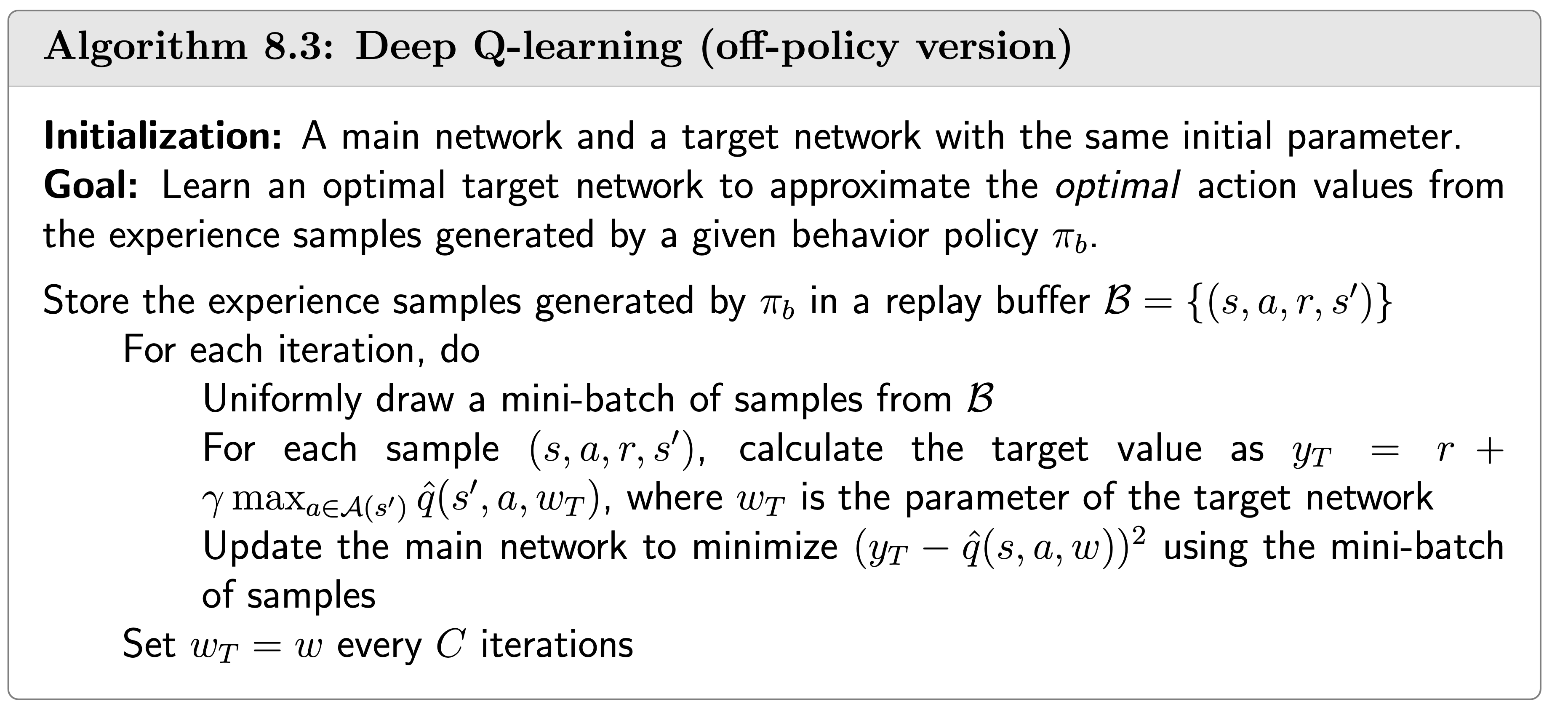
Implementation details: - Let \(w\) and \(w_T\) denote the parameters of the main and target networks, respectively. They are set to be the same initially.
In every iteration, we draw a mini-batch of samples \(\left\{\left(s, a, r, s^{\prime}\right)\right\}\) from the replay buffer (will be explained later).
The inputs of the networks include state \(s\) and action \(a\). The target output is \[ y_T \doteq r+\gamma \max _{a \in \mathcal{A}\left(s^{\prime}\right)} \color{red}{\hat{q}\left(s^{\prime}, a, w_T\right)} . \] Then, we directly minimize the TD error or called loss function \(\left(y_T-\hat{q}(s, a, w)\right)^2\) over the mini-batch \(\left\{\left(s, a, y_T\right)\right\}\).
As in Q learning, the action used in \(\hat{q}(s, a, w)\) is called the current action, and the action used in \(\hat{q}\left(s, a, w_T\right)\) (or \(y_T\)) is called the target action.
Replay buffer
Replay buffer (or experience replay in the original paper) is used in DQN to make the samples i.i.d.
1 | from collections import deque |
Pesudocode of DQN
Target network
Firstly, it is possible to build a DQN with a single Q Network and no Target Network. In that case, we do two passes through the Q Network, first to output the Predicted Q value, and then to output the Target Q value.
But that could create a potential problem. The Q Network’s weights get updated at each time step, which improves the prediction of the Predicted Q value. However, since the network and its weights are the same, it also changes the direction of our predicted Target Q values. They do not remain steady but can fluctuate after each update. This is like chasing a moving target.
By employing a second network that doesn’t get trained, we ensure that the Target Q values remain stable, at least for a short period. But those Target Q values are also predictions after all and we do want them to improve, so a compromise is made. After a pre-configured number of time-steps, the learned weights from the Q Network are copied over to the Target Network.
This is like EMA?
DQN
1 | class DQN(nn.Module): |
Loss
1 | def compute_td_loss(batch_size, replay_buffer, model, gamma, optimizer): |
Training process
1 | num_frames = 10000 |
OKay I know this explanation is ridiculous. In my opinion, the true reason of we favoring DQN over Q-learning with function approximation is simply the fact that DQN works better.↩︎