SimCLR

Sources:

1. SimCLR v1 2020 paper
2. SimCLR v2 2020 paper
3. Contrastive Representation Learning by Lilian
4. UVA's SimCLR implementation(Both Pytorch and Jax versions are implemented)

Introduction of contrastive learning

Self-supervised Learning is the technique of learning rich useful representations out of unlabelled data which can then be used for downstream tasks i.e. use it as initialization and finetune(either the whole network or only the linear classifier) the network on limited data.

Contrastive learning is one of many Self-supervised Learning paradigms that fall under Deep Distance Metric Learning where the objective is to learn a distance in a low dimensional space which is consistent with the notion of semantic similarity. In simple terms(considering image domain), it means to learn similarity among images where distance is less for similar images and more for dissimilar images.

Gist of the approach:

1. Create similar and dissimilar sets for every image in the dataset.
2. Pass two images(from similar/dissimilar set) to the same neural network and extract low dimensional embeddings/representations.
3. Compute euclidean distance between both the embeddings (not pixels!).
4. Minimize loss such that the above objective is achieved.
5. Repeat 1–4 for large number of pairs(all pairs may be infeasible) until the model converges.

SimCLR

SimCLR is a very simple framework for unsupervised pretraining. It learns representations by maximizing agreement between differently augmented views of the same data example via a contrastive loss in the latent space (not in the pixel space).

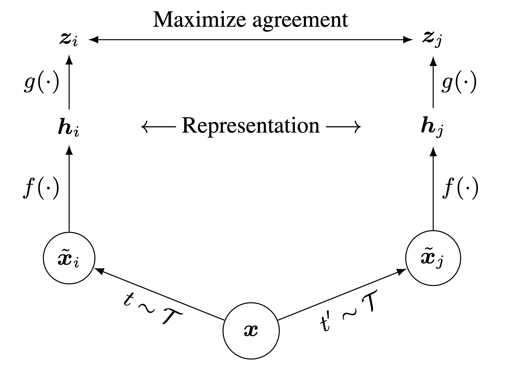
As illustrated in Figure 1, SimCLR comprises the following four major components.

1. A stochastic data augmentation family $$. We sample two separate data augmentation operators from it $(t\sim \mathcal{T}$ and $t^{\prime }\sim \mathcal{T}$), and apply them to each data example to obtain two correlated views denoted ${\tilde{\mathit{x}}}_i$ and ${\tilde{\mathit{x}}}_j$..

2. A neural network encoder $f(\cdot )$ (ResNet in practice) that extracts representation vectors from augmented data examples. $${\mathit{h}}_i=f\left({\tilde{\mathit{x}}}_i\right)=\mathrm{ResNet}\left({\tilde{\mathit{x}}}_i\right)$$ where ${\mathit{h}}_i\in {\mathbb{R}}^d$ is the output after the average pooling layer.

3. A small neural network projection head $g(\cdot )$ (2-3 layers MLP in practice) that maps representations to the latent space where contrastive loss is applied. $${\mathit{z}}_i=g\left({\mathit{h}}_i\right)$$

4. A contrastive loss function. Given a set $\left\{{\tilde{\mathit{x}}}_k\right\}$ including a positive pair of examples ${\tilde{\mathit{x}}}_i$ and ${\tilde{\mathit{x}}}_j$, the contrastive prediction task aims to identify ${\tilde{\mathit{x}}}_j$ in ${\left\{{\tilde{\mathit{x}}}_k\right\}}_{k\ne i}$ for a given ${\tilde{\mathit{x}}}_i$.

Training process

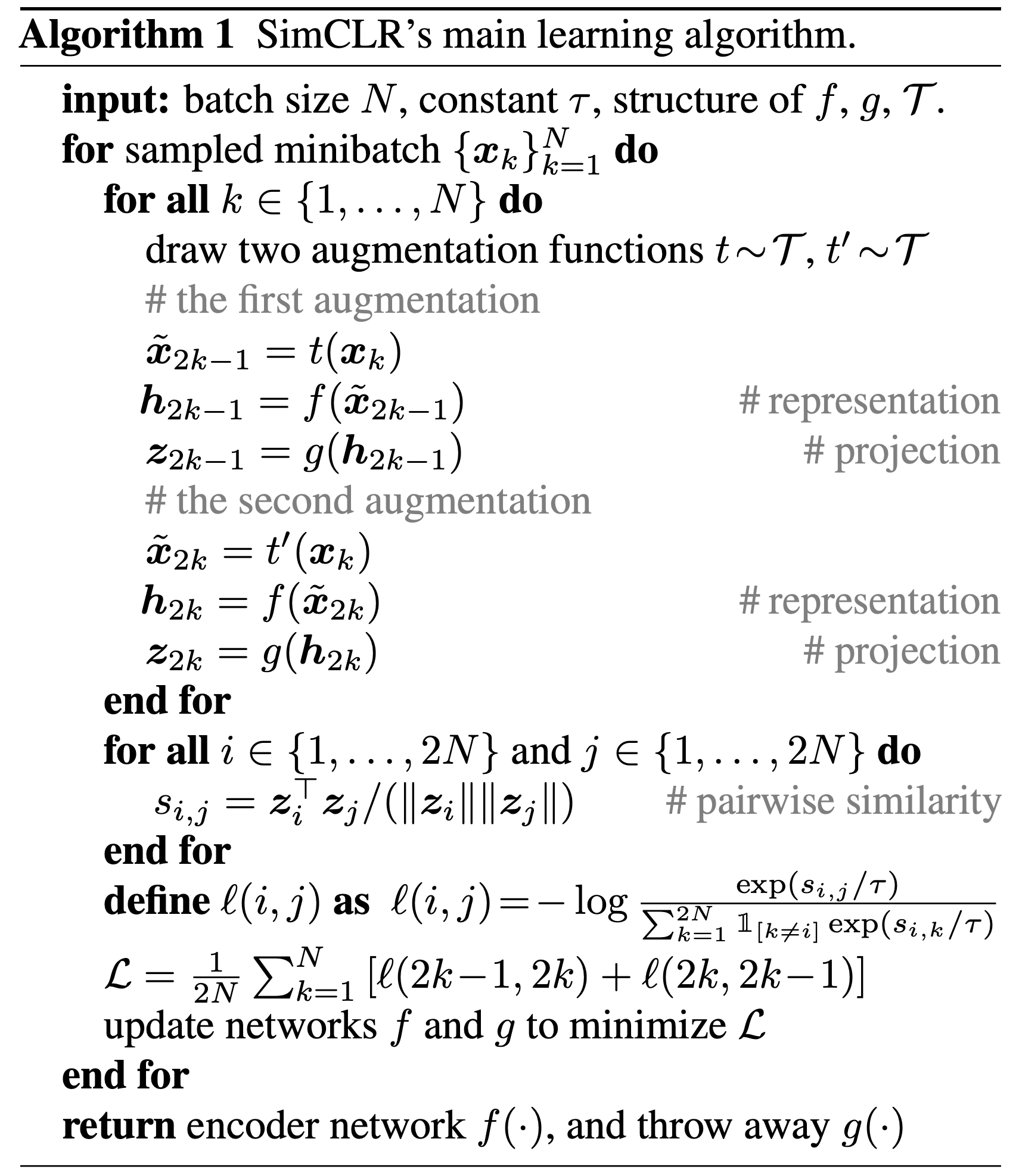
We randomly sample a minibatch of N examples, apply augmentation functions t(·) and t'(·) to them, resulting in 2N image views.

For each image, we construct positive and negative examples, which will be used in contrastive learning, as follows:

1. For each original image, we augment it into two views i and j. These views i and j are mutually positive examples.
2. All other 2(N-1) views k where k ≠ i and k ≠ j are negative examples of i (or j). Therefore, for each view i, we want to maximize its similarity with its positive example j, while minimizing its similarity to all negative examples k.

SimCLR proposes a NT-Xent loss (the normalized temperature-scaled cross entropy loss), which took inspiration from the InfoNCE loss, for contrastive learning. In short, the InfoNCE loss compares the similarity of $z_i$ and $z_j$ to the similarity of $z_i$ to any other representation in the batch by performing a softmax over the similarity values. The loss can be formally written as: $$\begin{array}{}\text{(1)}& {\ell }_{i,j}=-\log \frac{\exp \left(\mathrm{sim}({\mathit{z}}_i,{\mathit{z}}_j)/\tau \right)}{\sum _{k=1}^{2N}{\mathbb{1}}_{[k\ne i]}\exp \left(\mathrm{sim}({\mathit{z}}_i,{\mathit{z}}_k)/\tau \right)}\end{array}$$ where ${\mathbb{1}}_{[k\ne i]}\in \{0,1\}$ is an indicator function evaluating to 1 iff $k\ne i$ and $\tau$​ denotes a temperature parameter, and $\mathrm{sim}(\cdot )$ denotse the cosine similarity.

The final loss is computed across all positive pairs, both $(i,j)$ and $(j,i)$, in a mini-batch.

We can further derive $\text{(1)}$ into $$\begin{array}{}\text{(2)}& {\ell }_{i,j}=-\mathrm{sim}(z_i,z_j)/\tau +\log [\sum _{k=1}^{2N}{\mathbb{1}}_{[k\ne i]}\exp \left(\mathrm{sim}(z_i,z_k)/\tau \right)]\end{array}$$ for the ease of computation.

See the appendix for the implementation.

The exploration of compositions of data augmentation operations

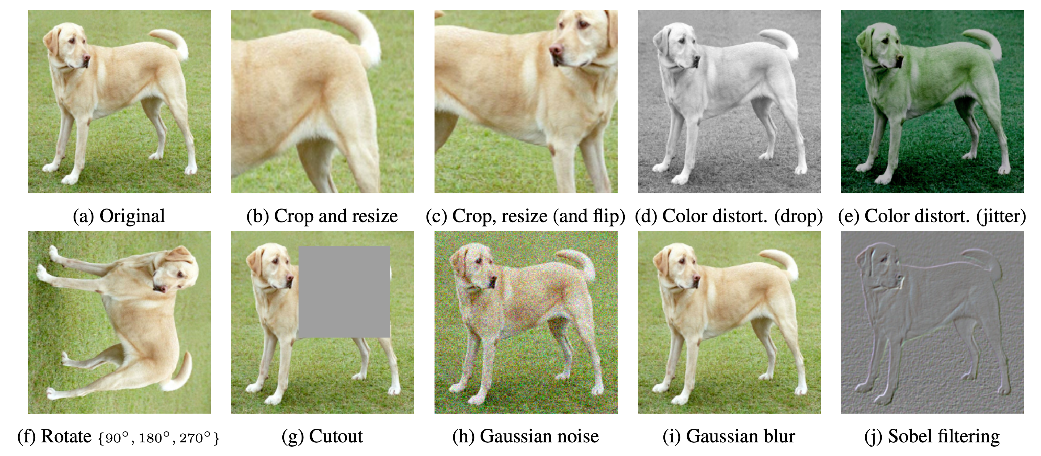
Composition of data augmentation operations is crucial for learning good representations. Figure 3 illustrates the studied data augmentation operators. Each augmentation can transform data stochastically with some internal parameters (e.g. rotation degree, noise level).

Note that we only test these operators in ablation, the augmentation policy used to train our models only includes random crop (with flip and resize), color distortion, and Gaussian blur.

The result of the ablation experiment is shown in Figure 4, where we tabulate the ImageNet top-1 accuracy under individual or composition of data augmentations, applied only to one branch.

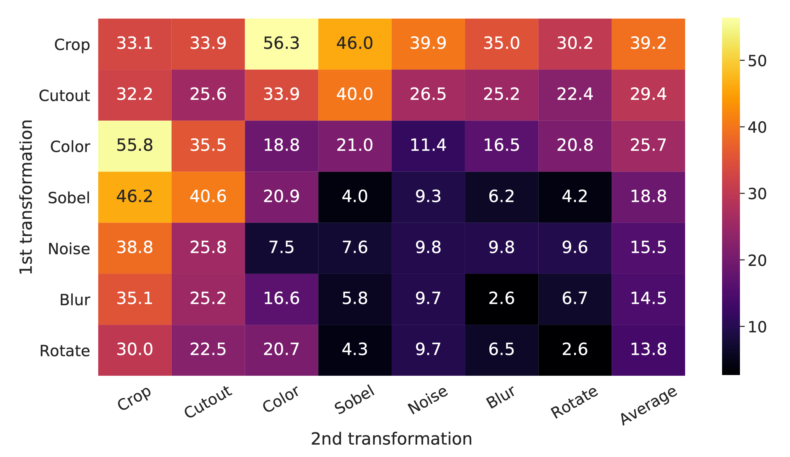
For all columns but the last, diagonal entries correspond to single transformation, and off-diagonals correspond to composition of two transformations (applied sequentially). The last column reflects the average over the row.

One composition of augmentations stands out: random cropping and random color distortion (acchieves accuray 55.8 or 56.3). We conjecture that one serious issue when using only random cropping as data augmentation is that most patches from an image share a similar color distribution.

Figure 4 shows that color histograms alone suffice to distinguish images. Neural nets may exploit this shortcut to solve the predictive task. Therefore, it is critical to compose cropping with color distortion in order to learn generalizable features.

Figure 5

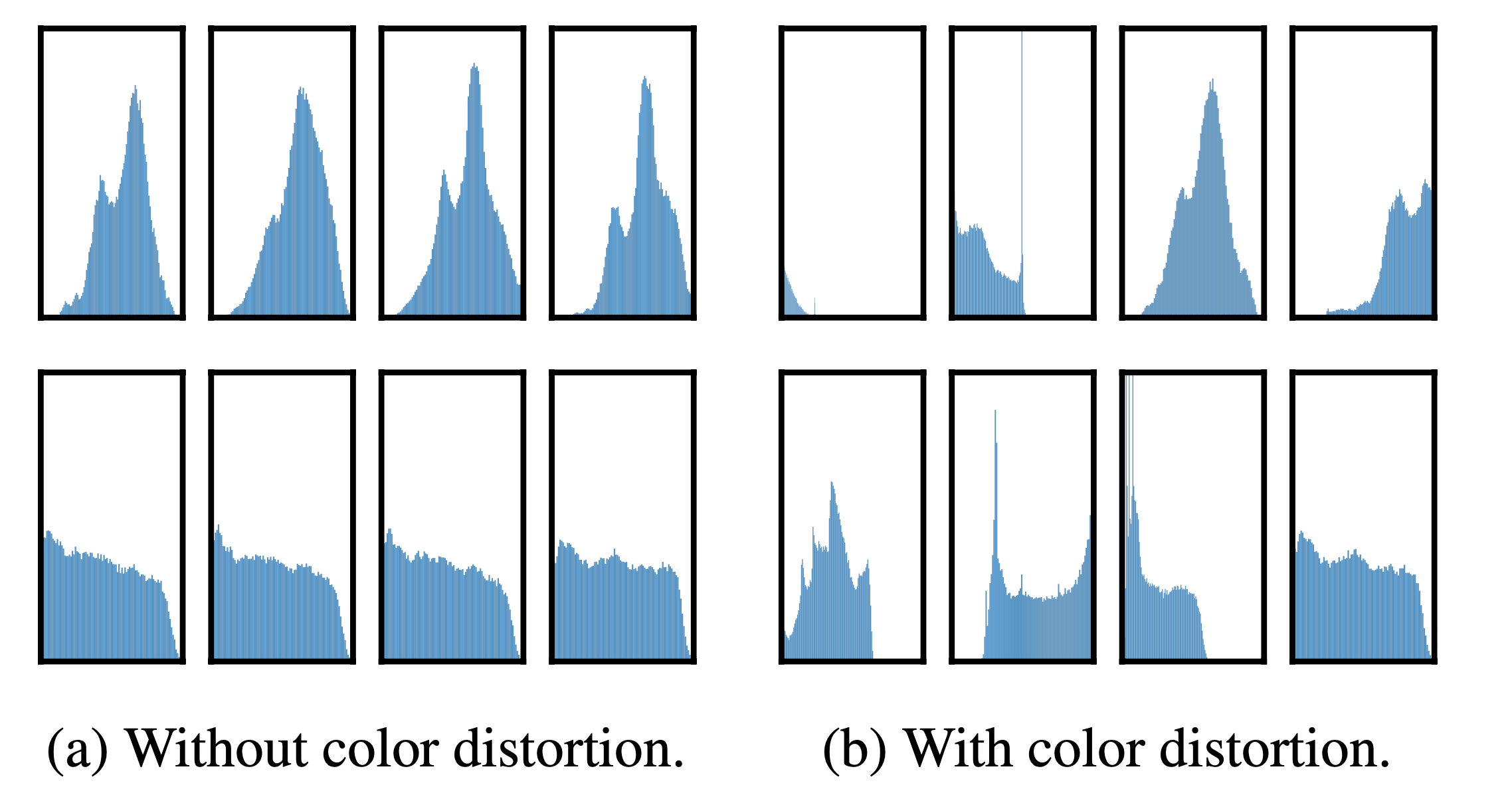
Figure 5. Histograms of pixel intensities (over all channels) for different crops of two different images (i.e. two rows). The image for the first row is from Figure 3. All axes have the same range.

SimCLR v2

SimCLR v2 is the successor of SimCLR. Basically it leverages bigger and deeper neural networks (bigger ResNets and MLPs) as its backbone. Meanwhile, it provides a three-stage pipeline for semi-supervised learning:

1. (unsupervised) pretraining
2. (supervised) fine-tune
3. (supervised) distill

Figure 6

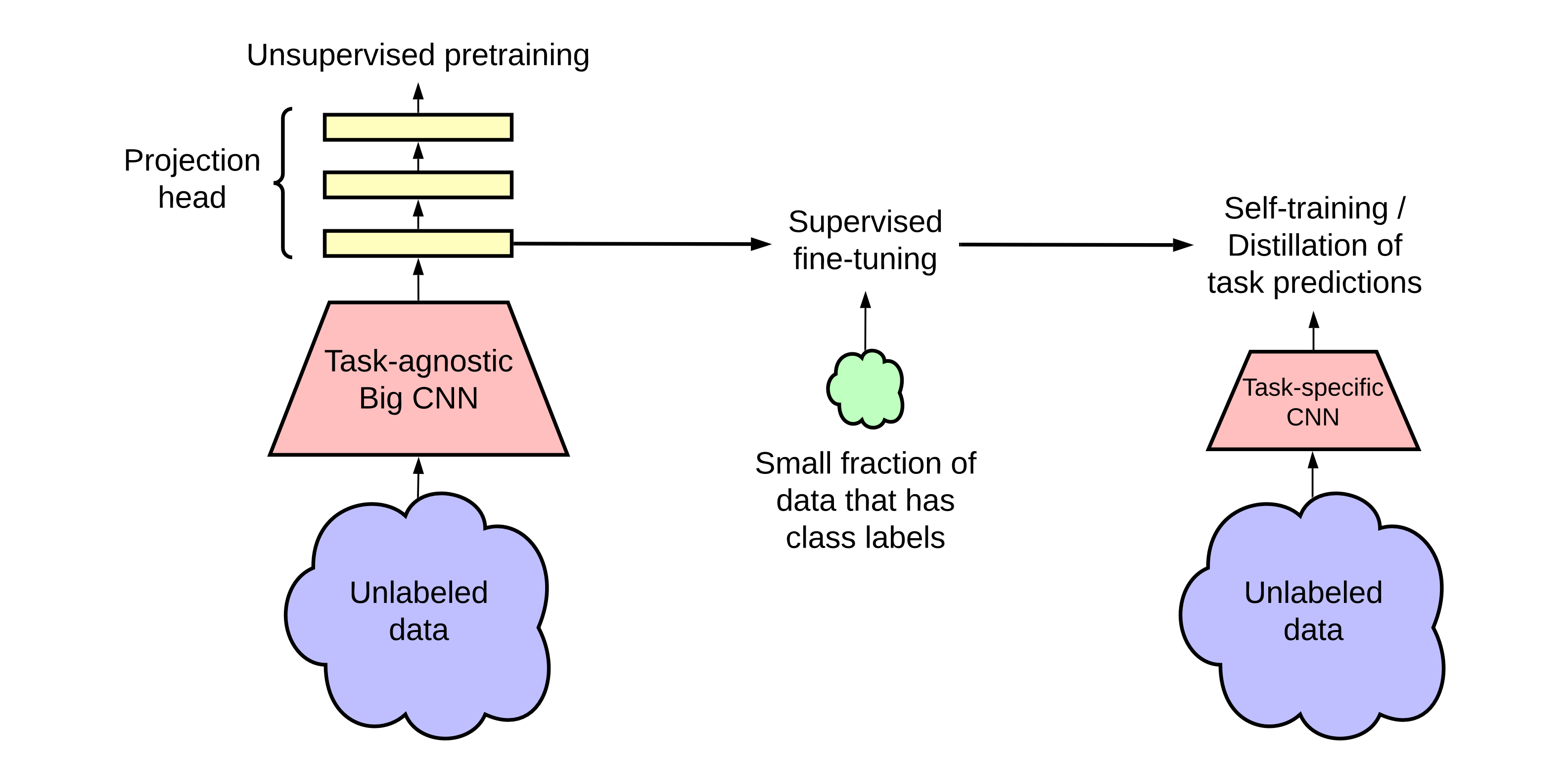
We then illustrate the process of knowledge distillation via unlabeled examples. To further improve the network for the target task, we use the fine-tuned network as a teacher to impute labels for training a student network. Specifically, we minimize the following distillation loss where no real labels are used: $${\mathcal{L}}^{\text{distill }}=-\sum _{{\mathit{x}}_i\in \mathcal{D}}[\sum _y{P}^T(y\mid {\mathit{x}}_i;\tau )\log P^S(y\mid {\mathit{x}}_i;\tau )]$$ where $$P(y\mid {\mathit{x}}_i)=\exp (f^{\text{task }}\left({\mathit{x}}_i\right)[y]/\tau )/\sum _{y^{\prime }}\exp \left(f^{\text{task }}\left({\mathit{x}}_i\right)\left[y^{\prime }\right]/\tau \right),$$ and $\tau$ is a scalar temperature parameter.

The teacher network, which produces $P^T(y\mid {\mathit{x}}_i)$, is fixed during the distillation; only the student network, which produces $P^S(y\mid {\mathit{x}}_i)$, is trained.

While we focus on distillation using only unlabeled examples in this work, when the number of labeled examples is significant, one can also combine the distillation loss with ground-truth labeled examples using a weighted combination $$\mathcal{L}=-(1-\alpha )\sum _{({\mathit{x}}_i,y_i)\in {\mathcal{D}}^L}[\log P^S(y_i\mid {\mathit{x}}_i)]-\alpha \sum _{{\mathit{x}}_i\in \mathcal{D}}[\sum _y{P}^T(y\mid {\mathit{x}}_i;\tau )\log P^S(y\mid {\mathit{x}}_i;\tau )].$$

This procedure can be performed using students either with the same model architecture (selfdistillation), which further improves the task-specific performance, or with a smaller model architecture, which leads to a compact model.

Appendix

InfoNCE loss

Suppose we have $N$ images in the dataset, during the training process, we

Suppose that we extract $B$ images from the dataset (or dataloader) each time, for an image $x_i$ in the dataset, $i\in \{1,\cdots ,B\}$, we apply transformations transformations $f(\cdot )$ and $g(\cdot )$ to it, resulting in 2 transformed image views, denoted as $x_i^1,x_i^2$.

Since there are $B$ images in the batch, the amount of transformed image views generated from the batch is $2B$.

Now we make those $2B$ image views as a new batch with batch size $B^{\prime }=2B$, we regulate that, for any image $x_i$, its views $x_i^1$ and $x_i^2$ are spaced by $B^{\prime }/2=B$ in the new batch, such that the new batch is like $$[x_1^1,x_2^1,\cdots ,x_B^1,x_1^2,x_2^2,\cdots ,x_B^2]$$ After that, we use the same neural network (typically a ResNet), denoted as function $f(\cdot )$, to map all $x_i^1,x_i^2$ into $z_i^1,z_i^2$. Note that here I use different notation from $\text{(???)}$, resulting in $$[z_1^1,z_2^1,\cdots ,z_B^1,z_1^2,z_2^2,\cdots ,z_B^2]$$ Now that, by the definition of InfoNCE loss, we want to make $\mathrm{sim}(z_i^1,z_i^2)$ smaller, while making $\mathrm{sim}(z_i^p,z_j^q)$ larger, where $i\ne j$, $p,q\in \{1,2\}$, $p$ and $q$ can be equal or different.

In contrastive learning, $z_i^1$ and $z_i^2$ (or $x_i^1$ and $x_i^2$) form a positive pair, whereas $z_i^p$ and $z_j^q$ (or $x_i^p$ and $x_j^q$) form a negative pair.

Since we have regulated that, in the new batch, $z_i^1$ and $z_i^2$ are spaced by $B$ indices, we can easily find positive pairs for any $z_i^1$, and the left pairs become all negative pairs naturally.

For example, soppose $B=2$ and $B^{\prime }=4$, the computation is as follows:

1. Get the cosine similarity matrix (and scale it by a temperature parameter):

   cos_sim = [
       [s11, s12, s13, s14],
       [s21, s22, s23, s24],
       [s31, s32, s33, s34],
       [s41, s42, s43, s44]
   ]

2. For numerical stabily, the diagonal of the cosine similarity matrix is set to a very low value

   cos_sim = [
       [-inf, s12, s13, s14],
       [s21, -inf, s23, s24],
       [s31, s32, -inf, s34],
       [s41, s42, s43, -inf]
   ]

3. Here, $z_1^1$ is indexed by 1, $z_1^2$ is indexed by 1+B=3. So the similarity of the first positive pair is s13. For the same reason, we can get the similarity of all the positive pairs

   s13, s24, s31, s42

   Threfore, the similarity of all the negative pairs are

   -inf, s12, s14, s21, -inf, s23, s32, -inf, s34, s41, s43, -inf

   To extract them, we simply make two index arrays:

   diag_range = [1, 2, 3, 4]
   shifted_diag_range = [1+B % B', 2+B % B', 3+B % B', 4+B % B'] = [3, 4, 1, 2]

   Extract the positive pairs with these indices:

   positive_pair_sim_array = cos_sim[diag_range, shifted_diag_range]
   '''
   Get: s13, s24, s31, s42
   '''

4. From $\text{(2)}$, we compute the InfoNCE loss from the similarity of positive pairs and negative pairs:

   nll = - positive_pair_sim_array + nn.logsumexp(cos_sim, axis=-1)
   nll = nll.mean()