Some Useful Signal Models
Sources:
- B. P. Lathi & Roger Green. (2021). Chapter 1: Signals and Systems. Signal Processing and Linear Systems (2nd ed., pp. 64-136). Oxford University Press.
- James McClellan, Ronald Schafer & Mark Yoder. (2015). Sinusoids. DSP First (2nd ed., pp. 9-40). Pearson.
The unit step function
The continuous-time unit step function \(u(t)\)
Definition: The unit step function, \(u(t)\), is defined as \[ u(t)= \begin{cases}0 & t<0 \\ 1 & t \ge 0\end{cases} \]
The discrete-time unit impulse function \(u[n]\)
\[ u[n]=\left\{\begin{array}{ll} 0, & n<0 \\ 1, & n \geq 0 \end{array} .\right. \]
The rectangular pulse
A common situation in a circuit is for a voltage to be applied at a particular time (say \(t=a\) ) and removed later at \(t=b\) (say). We write such a situation using unit step functions as: \[ x(t)=u(t-a)-u(t-b) \]
This voltage has strength 1 , duration \((b-a)\).
The unit impulse function
The continuous-time unit mpulse function \(\delta (t)\)
Definition: The unit impulse function, \(\delta(t)\), is defined in two parts by P. A. M. Dirac as \[ \begin{equation} \label{eq_1.9} \delta(t)=0 \quad t \neq 0 \quad \text { and } \quad \int_{-\infty}^{\infty} \delta(t) d t=1 \end{equation} \]
\(\delta(t)=0\) everywhere except at \(t=0\), where it is undefined.
We can visualize an impulse as a tall, narrow, rectangular pulse of unit area, as illustrated in Fig. 1.19b.
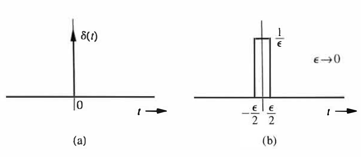
The width of this rectangular pulse is a very small value \(\epsilon \rightarrow 0\). Consequently, its height is a very large value \(1 / \epsilon \rightarrow \infty\). The unit impulse therefore can be regarded as a rectangular pulse with a width that has become infinitesimally small, a height that has become infinitely large, and an overall area that has been maintained at unity.
Since \(\delta (t)\) is undefined at \(t=0,\) a unit impulse is represented by the spearlike symbol in Fig. 1.19a.
The discrete-time unit impulse function \(\delta[n]\)
\[ \delta[n]= \begin{cases}0, & n \neq 0 \\ 1, & n=0\end{cases} \]
Multiplication of a function by an impulse
Let us now consider what happens when we multiply the unit impulse \(\delta(t)\) by a function \(\phi(t)\) that is known to be continuous at \(t=0\). Since the impulse has nonzero value only at \(t=0\), and the value of \(\phi(t)\) at \(t=0\) is \(\phi(0)\), we obtain \[ \phi(t) \delta(t)=\phi(0) \delta (t) \]
which equals to \(\phi(0)\) .
We can generalize this result. Say that provided \(\phi(t)\) is continuous at \(t=T\), \(\phi(t)\) multiplied by an impulse \(\delta(t-T)\) (impulse located at \(t=T)\) results in: \[ \begin{equation} \label{eq_1.10} \color {brown} {\phi(t) \delta(t-T)=\phi(T) \delta(t-T)} \end{equation} \]
which equals to $ (T)$.
Meanwhile, we also have \[ \phi(t) \delta(T-t)=\phi(T) \delta(T-t) \] The profe is rather simple. Considering \(\phi(t) \delta(T-t)\), we can use a change of variables to understand this expression. Let \(u=T-t\), then \(t=T-u\). The delta function \(\delta(T-t)\) can be rewritten as \(\delta(u)\), since \(\delta(x)=\) \(\delta(-x)\). Thus, we have: \[ \phi(t) \delta(T-t)=\phi(T-u) \delta(u) = \phi(T) \delta(u) = \phi(T) \delta(T-t) . \]
Q.E.D.
Sampling property of the unit impulse function
From \(\eqref{eq_1.10}\) it follows that \[ \begin{align} & \int_{-\infty}^{\infty} \color {brown} {\phi(t) \delta(t-T) d t} \label{eq_1.11} \\ & = \int_{-\infty}^{\infty} \color {brown} {\phi(T) \delta(t-T) d t} \\ & =\phi(T) \int_{-\infty}^{\infty} \delta(t) d t \nonumber \\ & = \color{red} {\phi(T)} \nonumber \end{align} \] provided \(\phi(t)\) is continuous at \(t=T\).
This property is very important and useful and is known as the sampling or sifting property of the unit impulse.
Unit impulse as a generalized function
The definition of the unit impulse function given in \(\eqref{eq_1.9}\) is not mathematically rigorous. It does not define a unique function, and it is undefined at \(t=0\).
These difficulties are resolved by defining the impulse as a generalized function of an impulse, rather than an ordinary function. A generalized function is defined by its effect on other functions instead of by its value at every instant of time.
Because the unit step function \(u(t)\) is discontinuous at \(t=0\), its derivative \(d u / d t\) does not exist at \(t=0\) in the ordinary sense. We now show that this derivative does exist in the generalized sense, and it is, in fact, \(\delta(t)\). As a proof, let us evaluate the integral of \((d u / d t) \phi(t)\), using integration by parts: \[ \begin{aligned} \int_{-\infty}^{\infty} \frac{d u(t)}{d t} \phi(t) d t & =\left.u(t) \phi(t)\right|_{-\infty} ^{\infty}-\int_{-\infty}^{\infty} u(t) {\phi}' (t) d t \\ & =\phi(\infty)-0-\int_0^{\infty} {\phi}' (t) d t \\ & =\phi(\infty)-\left.\phi(t)\right|_0 ^{\infty}=\phi(0) \end{aligned} \]
This result shows that \(d u / d t\) satisfies the sampling property of \(\delta(t)\). Therefore, it is an impulse \(\delta(t)\) in the generalized sense-that is, \[ \frac{d u(t)}{d t}=\delta(t) . \]
Consequently, # TODO \[ \int_{-\infty} ^{t} \delta(\tau) d \tau=u(t) . \]
We observe that the area from \(-\infty\) to \(t\) under the limiting form of \(\delta(t)\) in Fig. \(1.19 \mathrm{~b}\) is zero if \(t<-\epsilon / 2\) and unity if \(t \geq \epsilon / 2\) with \(\epsilon \rightarrow 0\). Consequently, \[ \begin{aligned} \int_{-\infty}^{t} \delta(\tau) d \tau & = \begin{cases}0 & t<0 \\ 1 & t \geq 0\end{cases} \\ & =u(t) \end{aligned} \]