Size of a Signal
Sources:
- B. P. Lathi & Roger Green. (2021). Chapter 1: Signals and Systems. Signal Processing and Linear Systems (2nd ed., pp. 64-136). Oxford University Press.
Introduction of signals
A signal is a set of data or information. In this serie, we focus our attention on signals involving a single independent variable. For convenience, we will generally refer to the independent variable as time, although it may not in fact represent time in specific applications.
Continuous-time and discrete-time signals
Throughout this serie we will be considering two basic types of signals:
- continuous-time signals, and
- discrete-time signals.
To distinguish between them, we will use the symbol \(t\) to denote the continuous-time independent variable and \(n\) to denote the discretetime independent variable.
In addition, for continuous-time signals we will enclose the independent variable in parentheses \((\cdot)\), whereas for discrete-time signals we will use brackets \([\cdot]\) to enclose the independent variable.
For further emphasis we will on occasion refer to \(x[n]\) as a discrete-time sequence.
Signal energy
We may consider the area under a signal \(x(t)\) as a possible measure of its size, because it takes account not only of the amplitude but also of the duration. However, this will be a defective measure because even for a large signal \(x(t)\), its positive and negative areas could cancel each other, indicating a signal of small size.
This difficulty can be corrected by defining the signal size as the area under \(|x(t)|^2\), which is always positive. We call this measure the signal energy1 \(E_x\), defined as \[ \begin{equation} \label{eq_1.1} E_x=\int_{-\infty}^{\infty}|x(t)|^2 d t \end{equation} \]
This definition simplifies for a real-valued signal \(x(t)\) to \(E_x=\int_{-\infty}^{\infty} x^2(t) d t\).
There are also other possible measures of signal size, such as the area under \(|x(t)|\). The energy measure, however, is not only more tractable mathematically but is also more meaningful (as shown later) in the sense that it is indicative of the energy that can be extracted from the signal.
For discrete signal, the result is similar: \[ E_x=\sum_{n= -\infty}^{\infty}|x[n]|^2 . \]
Signal power
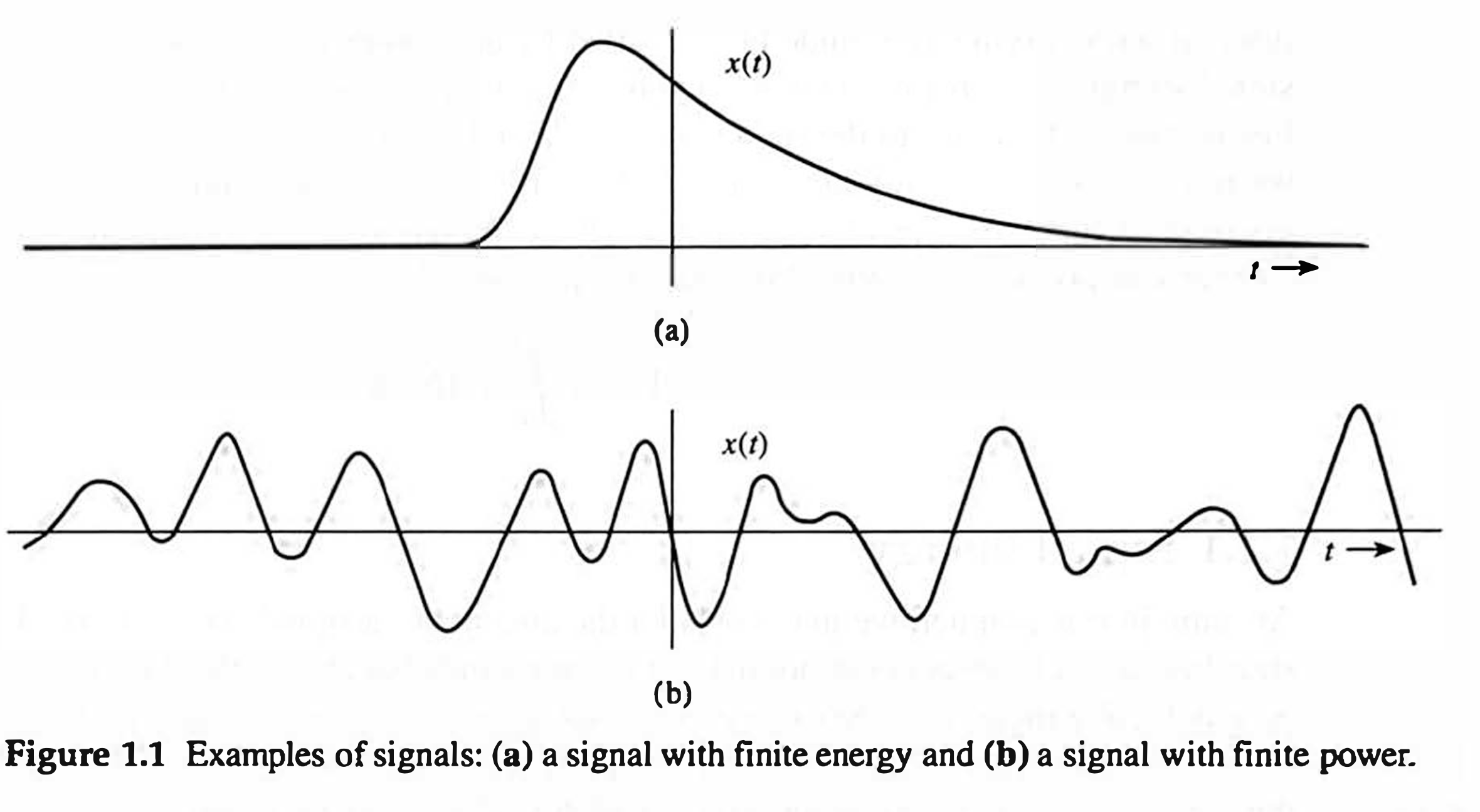
Signal energy must be finite for it to be a meaningful measure of signal size. A necessary condition for the energy to be finite is that the signal amplitude \(\rightarrow 0\) as \(|t| \rightarrow \infty\) (Fig. 1.1a). Otherwise, the integral in \(\eqref{eq_1.1}\) will not converge.
When the amplitude of \(x(t)\) does not \(\rightarrow 0\) as \(|t| \rightarrow \infty\) (Fig. 1.1b), the signal energy is infinite. A more meaningful measure of the signal size in such a case would be the time average of the energy, if it exists. This measure is called the power of the signal. For a signal \(x(t)\), we define its power \(P_x\) as \[ \begin{equation} \label{eq_1_2} \color{red} {P_x=\lim _{T \rightarrow \infty} \frac{1}{T} \int_{-T / 2}^{T / 2}|x(t)|^2 d t} . \end{equation} \]
This definition simplifies for a real-valued signal \(x(t)\) to \(P_x=\lim _{T \rightarrow \infty} \frac{1}{T} \int_{-T / 2}^{T / 2} x^2(t) d t\).
We also have a measurement called the root-mean-square (rms) value, it's just the square root of \(P_x\).
For discrete signal, \[ P_{x} \triangleq \lim _{N \rightarrow \infty} \frac{1}{2 N+1} \sum_{n=-N}^{+N}|x[n]|^2 \]
For periodic signals
For a periodic signal \(x(t)\) with minimum period \(T_0\), this equation can be formulated as \[ \color{blue} {P_x= \frac{1}{T_0} \int_{-T_0 / 2}^{T_0 / 2}|x(t)|^2 d t = \frac{1}{T_0} \int_{T_0} |x(t)|^2 d t} . \]
Proof:
Let \(T =n T_0\), \(n \in N\), we can easily prove \(T\) and \(n T_0\) are infinitesimals of the same order, then we obtain \[ P_x = \color{red} {\lim _{T \rightarrow \infty} \frac{1}{T} \int_{-T / 2}^{T / 2}|x(t)|^2 d t } = \lim _{n \rightarrow \infty} \frac{1}{n T_0} \int_{-\frac{n T_0}{2}}^{\frac{n T_0}{2}}|x(t)|^2 d t . \]
Because \(x(t)\) is periodic, \(|x(t)|^2\) is also periodic, according to this post, for periodoc signals, we have \[ {\int_a^{a+T_0} f(x) d x=\int_b^{b+T_0} f(x) d x } \] where \(a, b\) can be whatever value.
Thus, we get \[ \int_{-\frac{n T_0}{2}}^{\frac{n T_0} {2}}|x(t)|^2 d t =\int_0^{n T_0}|x(t)|^2 d t \] Now we do \[ \begin{aligned} \int_0^{n T_0}|x(t)|^2 d t & =\sum_{i=0}^{n-1} \int_{i T_0}^{(i+1) T_0}|x(t)|^2 d t \\ & =\sum_{i=0}^{n-1} \int_0^{T_0}|x(t)|^2 d t \\ & =n \int_0^{T_0}|x(t)|^2 d t . \end{aligned} \] As a result, \[ \begin{aligned} P_x & =\lim _{n \rightarrow \infty} \frac{1}{n T_0} \cdot n \cdot \int_0^{T_0}|x(t)|^2 d t \\ & =\lim _{n \rightarrow \infty} \frac{1}{T_0} \int_0 T_0|x(t)|^2 d t \\ & = \color{blue} {\frac{1}{T_0} \int_0^{T_0}|x(t)|^2 d t} . \end{aligned}, \] Q.E.D.
Example: Determining Power and RMS Value
Here we show that a sinusoid of amplitude \(C\) has a power \(C^2 / 2\) regardless of the value of its frequency \(\omega_0\) (when \(\omega_0 \neq 0\)) and phase \(\theta\).
- Prove that, for \[ x(t)=C \cos \left(\omega_0 t+\theta\right) , \]
we have \[ \begin{equation} \label{eq_a} \color{green} {P_x=\frac{C^2}{2}} \end{equation} \] for \(w_0 \neq 0\), and \(\color{green} {P_x = C^2}\) for \(w_0 = 0\).
- Prove that, for \[ x(t)=C_1 \cos \left(\omega_1 t+\theta_1\right)+C_2 \cos \left(\omega_2 t+\theta_2\right) \quad \omega_1 \neq \omega_2 , \]
we have \[ \begin{equation} \label{eq_b} \color{purple} {P_x=\frac{C_1^2}{2}+\frac{C_2^2}{2}} \end{equation} \] for \(\omega_1 \neq \omega_2 \neq 0\).
- Prove that, for \[ x(t)=D e^{j \omega_0 t} \]
we have \[ \begin{equation} \label{eq_c} \color{CarnationPink} {P_x=|D|^2} . \end{equation} \]
(a)
For \(w_0 \neq 0\), this is a periodic signal with period \(T_0=2 \pi / \omega_0\). The suitable measure of this signal is its power. Because it is a periodic signal, we may compute its power by averaging its energy over one period \(T_0=2 \pi / \omega_0\). However, for the sake of demonstration, we shall use \(\eqref{eq_1_2}\) to solve this problem by averaging over an infinitely large time interval. $$ \[\begin{aligned} P_x & =\lim _{T \rightarrow \infty} \frac{1}{T} \int_{-T / 2}^{T / 2} C^2 \cos ^2\left(\omega_0 t+\theta\right) d t=\lim _{T \rightarrow \infty} \frac{C^2}{2 T} \int_{-T / 2}^{T / 2}\left[1+\cos \left(2 \omega_0 t+2 \theta\right)\right] d t \\ & =\lim _{T \rightarrow \infty} \frac{C^2}{2 T} \int_{-T / 2}^{T / 2} d t+\lim _{T \rightarrow \infty} \frac{C^2}{2 T} \int_{-T / 2}^{T / 2} \cos \left(2 \omega_0 t+2 \theta\right) d t \\ & = C^2 / 2 + 0 \\ & = C^2 / 2 \end{aligned}\]$$
Thus, we have \(\eqref{eq_a}\)
The rms value is \(C / \sqrt{2}\).
Note that, for \(w_0 = 0\), we can easily know \(P_x = C^2\).
(b)
In future post we shall show that a sum of two sinusoids may or may not be periodic, depending on whether the ratio \(\omega_1 / \omega_2\) is a rational number. Therefore, the period of this signal is not known.
Hence, its power will be determined by averaging its energy over \(T\) seconds with \(T \rightarrow \infty\). Thus, $$ \[\begin{aligned} P_x= & \lim _{T \rightarrow \infty} \frac{1}{T} \int_{-T / 2}^{T / 2}\left[C_1 \cos \left(\omega_1 t+\theta_1\right)+C_2 \cos \left(\omega_2 t+\theta_2\right)\right]^2 d t \\ = & \lim _{T \rightarrow \infty} \frac{1}{T} \int_{-T / 2}^{T / 2} C_1{ }^2 \cos ^2\left(\omega_1 t+\theta_1\right) d t+\lim _{T \rightarrow \infty} \frac{1}{T} \int_{-T / 2}^{T / 2} C_2{ }^2 \cos ^2\left(\omega_2 t+\theta_2\right) d t \\ = & \frac{C_1^2}{2}+\frac{C_2^2}{2} . \end{aligned}\]$$
The first and second integrals on the right-hand side are the powers of the two sinusoids, which are \(C_1{ }^2 / 2\) and \(C_2{ }^2 / 2\), as found in part (a). The third term, the product of two sinusoids, can be expressed as a sum of two sinusoids \(\cos \left[\left(\omega_1+\omega_2\right) t+\left(\theta_1+\theta_2\right)\right]\) and \(\cos \left[\left(\omega_1-\omega_2\right) t+\left(\theta_1-\theta_2\right)\right]\), respectively. Now, arguing as in part (a), we see that the third term is zero. Hence, we have \(\eqref{eq_b}\)
and the rms value is \(\sqrt{\left(C_1{ }^2+C_2{ }^2\right) / 2}\).
We can readily extend this result to a sum of any number of sinusoids with distinct frequencies. Thus, if \[ x(t)=\sum_{n=1}^{\infty} C_n \cos \left(\omega_n t+\theta_n\right) \] assuming that none of the two sinusoids have identical frequencies and \(\omega_n \neq 0\), then \[ \color{purple} {P_x=\frac{1}{2} \sum_{n=1}^{\infty} C_n{ }^2} . \]
If \(x(t)\) also has a dc term, as \[ x(t)=C_0+\sum_{n=1}^{\infty} C_n \cos \left(\omega_n t+\theta_n\right) . \] then \[ \color{purple} {P_x=C_0^2+\frac{1}{2} \sum_{n=1}^{\infty} C_n^2 } . \]
(c)
In this case the signal is complex, and we use \(\eqref{eq_1_2}\) to compute the power. \[ P_x=\lim _{T \rightarrow \infty} \frac{1}{T} \int_{-T / 2}^{T / 2}\left|D e^{j \omega_0 t}\right|^2 \]
Recall that \(\left|e^{j \omega_0 t}\right|=1\)2 so that \(\left|D e^{j \omega_0 t}\right|^2=|D|^2\), and \(\eqref{eq_c}\).
The rms value is \(|D|\).