Vector Quantized Variational Autoencoders

Posted on 2024-04-07 Edited on 2025-11-16 In Research Views: 79

Sources:

Link: My VQ-VAE implementation on Github

Vector Quantized Variational Autoencoders

Notation

Symbol	Type	Explanation
$x, y, z$	$\in R$	Cartesian coordinates
$u, v, w$	$\in R$	General curvilinear coordinates
$r, ϕ, z$	$\in R$	Cylindrical coordinates
$R, θ, ϕ$	$\in R$	Spherical coordinates
$r$	$\in R^{3}$	Position vector
$\hat{x}, \hat{y}, \hat{z}$	$\in R^{3}$	Cartesian unit basis vectors
$\hat{r}, \hat{ϕ}, \hat{z}$	$\in R^{3}$	Cylindrical unit basis vectors
$\hat{R}, \hat{θ}, \hat{ϕ}$	$\in R^{3}$	Spherical unit basis vectors
$e_{u}, e_{v}, e_{w}$	$\in R^{3}$	Base vectors in the transformed coordinate system
$d l$	$\in R^{3}$	Differential displacement vector
$d l_{u}, d l_{v}, d l_{w}$	$\in R^{3}$	Differential displacement vectors along each coordinate
$d s$	$\in R^{3}$	Differential area vector
$d s_{u}, d s_{v}, d s_{w}$	$\in R^{3}$	Differential area vectors along each coordinate
$d V$	$\in R$	Differential volume element
$J$	$\in R^{3 \times 3}$	Jacobian matrix of the coordinate transformation
$\det J$	$\in R$	Determinant of the Jacobian matrix, used for volume scaling
$e_{u} \cdot (e_{v} \times e_{w})$	$\in R$	Scalar triple product of base vectors, equal to $\det J$
$\nabla$	Operator	Gradient operator

Introduction

This section is modified from the brilliant and compact introduction of VQ-VAE from Finite Scalar Quantization: VQ-VAE Made Simple

Vector quantization (VQ), initially introduced by Gray (1984), has recently seen a renaissance in the context of learning discrete representations with neural networks. Spurred by the success of VQ-VAE (Van Den Oord et al., 2017), Esser et al. (2020) and Villegas et al. (2022) showed that training an autoregressive transformer on the representations of a VQ-VAE trained with a GAN loss enables powerful image and video generation models, respectively.

At the same time, VQ has become popular component in image (Bao et al., 2021; Li et al., 2023) and audio (Baevski et al., 2019) representation learning, and is a promising building block for the next generation of multimodal large language models (Aghajanyan et al., 2022; Kim et al., 2023; Aghajanyan et al., 2023).

When training VQ-VAE, the goal is to learn a codebook $C$ whose elements induce a compressed, semantic representation of the input data (typically images). In the forward pass, an image $x$ is encoded into a representation $z$ (typically a sequence of feature vectors), and each vector in $z$ quantized to (i.e., replaced with) the closest vector in $C$ . The quantization operation is not differentiable. When training a VAE with VQ in the latent representation, Van Den Oord et al. (2017) use the straightthrough estimator (STE) (Bengio et al., 2013), copying the gradients from the decoder input to the encoder output, resulting in gradients to the encoder. Since this still does not produce gradients for the codebook vectors, they further introduce two auxiliary losses to pull the codeword vectors towards the (unquantized) representation vectors and vice-versa.

Components of VQ-VAE

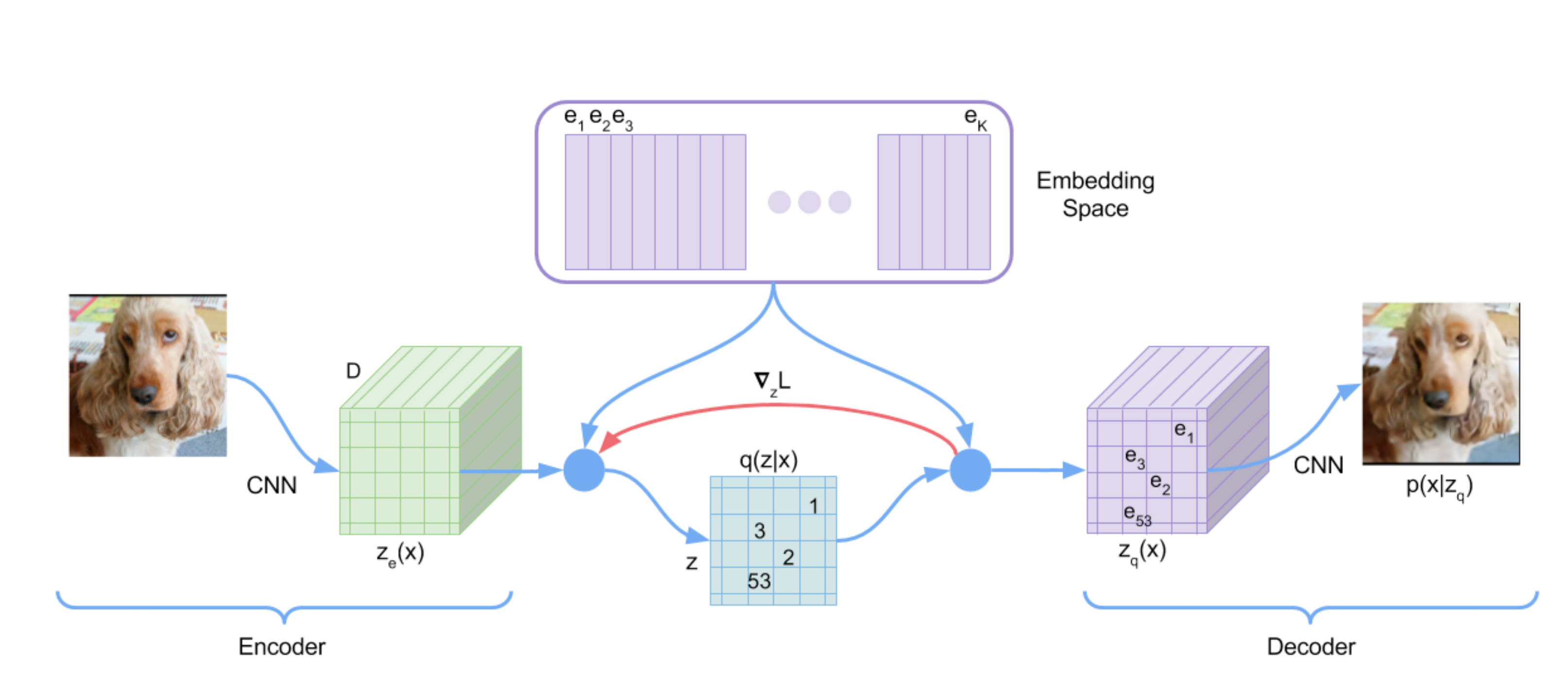
The Vector Quantised-Variational AutoEncoder (VQ-VAE), differs from VAEs in two key ways: the encoder network outputs discrete, rather than continuous, codes; and the prior is learnt rather than static.

In VQ-VAE, we have:

An input image $x \in R^{H \times W \times 3}$ where $H, W$ are the height and width of the image.
A latent embedding space $E = {e_{k}}_{k = 1}^{K} \subset R^{D}$ , called the codebook, where each $e_{k}$ is called a code and $D$ is the dimensionality of codes.
An encoder $\begin{aligned} (1) & E : R^{H \times W \times 3} \to R^{h \times w \times D} \\ (2) & E (x) = z_{e} \end{aligned}$ encodes an image $x$ into an embedding $z_{e}$ .
An operator called quantizer: $\begin{aligned} Qtzr : R^{h \times w \times D} \to R^{h \times w \times D} \\ Qtzr (z_{e}) = z_{q}, \end{aligned}$

quantizes $z_{e}$ to $z_{q}$ , where $z_{q}, z_{e} \in R^{h \times w \times D}$ . The quantization process is $z_{q_{i j}} = \arg min ‖ z_{e_{i j}} - e_{k} ‖$ with subscript $i, j$ starting from $1$ to $h, w$ .

Therefore, for each element $z_{e_{i j}}$ of $z_{e}$ , we use argmin to find the $e_{k}$ that is closest in distance to $z_{e_{i j}}$ , i.e., minimizing the norm $‖ z_{e_{i j}} - e_{k} ‖$ , to get $z_{q_{i, j}}$ .
A decoder $\begin{aligned} (3) & D : R^{h \times w \times D} \to R^{H \times W \times 3} \\ (4) & D (z_{q}) = \hat{x} \end{aligned}$ decodes $z_{q}$ into an image $\hat{x}$ , which is also called the reconstructed image of $x$ .

Forward pass

The forward pass of VQ-VAE consists of

First, we use encoder $E (.)$ to encode the input image $x$ to get the embedding $z_{e}$ : $z_{e} = E (x) .$
Next, we use quantizer $Qtzr (.)$ to quantize the embedding $z_{e}$ to get the quantized embedding $z_{q}$ . Since $z_{e}$ contains $h \times w$ embeddings, $z_{q}$ is composed of $h \times w$ codes, of which each code $e_{k}$ is selected through a nearest-neighbor lookup (argmin()) to the codebook $E = {e_{k}}_{k = 1}^{K}$ .
Finnally, we use decoder to decode $z_{e}$ to get the reconstructed image $\hat{x}$ .

NOTES:

The encoded embedding $z_{e}$ and quantized embedding $z_{q}$ have the same dimentionality $z_{e}, z_{q} \in R^{h \times w \times D} .$ and they have the same embedding dimenstion (= $D$ ) as $e_{k}$ .
We will sometimes use $z_{e} (x), z_{q} (x)$ to refer $z_{e}, z_{q}$ .

Loss function

The overall loss function is: $L = - \log p (x ∣ z_{q}) + {‖ sg (z_{e} - z_{q}) ‖}_{2}^{2} + β {‖ z_{e} - sg (z_{q}) ‖}_{2}^{2},$ Since VQ-VAE leverages argmin() function, which is non-differentiable. The gradient $\nabla_{z_{q}} L$ from decoder input $z_{q}$ can not be passed to the encoder output $z_{e}$ . To solve this, we use a trick called the straight through estimator which applies a stop_gradient operator ( $sg$ in the equation) to copy $\nabla_{z_{q}} L$ to $z_{e}$ .

The overall loss function has three components:

Reconstruction loss $- \log p (x ∣ z_{q})$ is the negative log-likelihood. In practice, it's common to replace it with MSE loss.
Codebook loss ${‖ sg [z_{e} (x)] - e ‖}_{2}^{2}$ , which moves the embedding vectors towards the encoder output.
Commitment loss $β {‖ z_{e} (x) - sg [e] ‖}_{2}^{2}$ , which encourages the encoder output to stay close to the embedding space.

Model architecture

#TODO shape problem

VectorQuantizer

This layer takes a tensor to be quantized. The channel dimension will be used as the space in which to quantize. All other dimensions will be flattened and will be seen as different examples to quantize.

The output tensor will have the same shape as the input.

As an example for a BCHW tensor of shape [16, 64, 32, 32], we will first convert it to an BHWC tensor of shape [16, 32, 32, 64] and then reshape it into [16384, 64] and all 16384 vectors of size 64 will be quantized independently. In otherwords, the channels are used as the space in which to quantize.

All other dimensions will be flattened and be seen as different examples to quantize, 16384 in this case.

class VectorQuantizer(nn.Module):
    def __init__(self, num_embeddings, embedding_dim, commitment_cost):
        super(VectorQuantizer, self).__init__()
        
        self._embedding_dim = embedding_dim
        self._num_embeddings = num_embeddings
        
        self._embedding = nn.Embedding(self._num_embeddings, self._embedding_dim)
        self._embedding.weight.data.uniform_(-1/self._num_embeddings, 1/self._num_embeddings)
        self._commitment_cost = commitment_cost

    def forward(self, inputs):
        # convert inputs from BCHW -> BHWC
        inputs = inputs.permute(0, 2, 3, 1).contiguous()
        input_shape = inputs.shape
        
        # Flatten input
        flat_input = inputs.view(-1, self._embedding_dim)
        
        # Calculate distances
        distances = (torch.sum(flat_input**2, dim=1, keepdim=True) 
                    + torch.sum(self._embedding.weight**2, dim=1)
                    - 2 * torch.matmul(flat_input, self._embedding.weight.t()))
            
        # Encoding
        encoding_indices = torch.argmin(distances, dim=1).unsqueeze(1)
        encodings = torch.zeros(encoding_indices.shape[0], self._num_embeddings, device=inputs.device)
        encodings.scatter_(1, encoding_indices, 1)
        
        # Quantize and unflatten
        quantized = torch.matmul(encodings, self._embedding.weight).view(input_shape)
        
        # Loss
        e_latent_loss = F.mse_loss(quantized.detach(), inputs)
        commitment_loss = self._commitment_cost * e_latent_loss
        codebook_loss = F.mse_loss(quantized, inputs.detach())
        
        
        quantized = inputs + (quantized - inputs).detach()
        avg_probs = torch.mean(encodings, dim=0)
        perplexity = torch.exp(-torch.sum(avg_probs * torch.log(avg_probs + 1e-10)))
        
        # convert quantized from BHWC -> BCHW
        return codebook_loss, commitment_loss, quantized.permute(0, 3, 1, 2).contiguous(), perplexity, encodings

We will also implement a slightly modified version which will use exponential moving averages to update the embedding vectors instead of an auxillary loss. This has the advantage that the embedding updates are independent of the choice of optimizer for the encoder, decoder and other parts of the architecture. For most experiments the EMA version trains faster than the non-EMA version.

VectorQuantizerEMA

class VectorQuantizerEMA(nn.Module):
    def __init__(self, num_embeddings, embedding_dim, commitment_cost, decay, epsilon=1e-5):
        super(VectorQuantizerEMA, self).__init__()
        
        self._embedding_dim = embedding_dim
        self._num_embeddings = num_embeddings
        
        self._embedding = nn.Embedding(self._num_embeddings, self._embedding_dim)
        self._embedding.weight.data.normal_()
        self._commitment_cost = commitment_cost
        
        self.register_buffer('_ema_cluster_size', torch.zeros(num_embeddings))
        self._ema_w = nn.Parameter(torch.Tensor(num_embeddings, self._embedding_dim))
        self._ema_w.data.normal_()
        
        self._decay = decay
        self._epsilon = epsilon

    def forward(self, inputs):
        # convert inputs from BCHW -> BHWC
        inputs = inputs.permute(0, 2, 3, 1).contiguous() # (256, 64, 8, 8) BCHW --> (256, 8, 8, 64) BHWC
        input_shape = inputs.shape # BHWC
        
        # Flatten input
        flat_input = inputs.view(-1, self._embedding_dim) # Now set C'=64 (_embedding_dim), flatten `inputs` into (N, C'), where N=B*H*W, i.e., we have N=B*H*W vectors, each vector has dimension=C.
        
        # Calculate distances
        distances = (torch.sum(flat_input**2, dim=1, keepdim=True) 
                    + torch.sum(self._embedding.weight**2, dim=1)
                    - 2 * torch.matmul(flat_input, self._embedding.weight.t())) # Each vector `z_e` has distances with all the quantized vectors `e_j` in the codebook, where j in K = `_num_embeddings`.
            
        # Encoding
        encoding_indices = torch.argmin(distances, dim=1).unsqueeze(1)# For each vector `z_e`, select the index of the **closest** quantized vector `e_j` in the codebook.
        
        # For each each vector `z_e`, use the index of its corresponding  `z_q` to create a one-hot encoding.
        encodings = torch.zeros(encoding_indices.shape[0], self._num_embeddings, device=inputs.device)
        encodings.scatter_(1, encoding_indices, 1)
        
        # Quantize and unflatten
        quantized = torch.matmul(encodings, self._embedding.weight).view(input_shape) # Use the one-hot encoding as the index to select the quantized vectors in the codebook.
        
        # Use EMA to update the embedding vectors
        if self.training:
            self._ema_cluster_size = self._ema_cluster_size * self._decay + \
                                     (1 - self._decay) * torch.sum(encodings, 0)
            
            # Laplace smoothing of the cluster size
            n = torch.sum(self._ema_cluster_size.data)
            self._ema_cluster_size = (
                (self._ema_cluster_size + self._epsilon)
                / (n + self._num_embeddings * self._epsilon) * n)
            
            dw = torch.matmul(encodings.t(), flat_input)
            self._ema_w = nn.Parameter(self._ema_w * self._decay + (1 - self._decay) * dw)
            
            self._embedding.weight = nn.Parameter(self._ema_w / self._ema_cluster_size.unsqueeze(1))
        
        # Loss
        e_latent_loss = F.mse_loss(quantized.detach(), inputs)
        commitment_loss = self._commitment_cost * e_latent_loss
        codebook_loss = F.mse_loss(quantized, inputs.detach())
        
        # Straight Through Estimator
        quantized = inputs + (quantized - inputs).detach()
        avg_probs = torch.mean(encodings, dim=0)
        perplexity = torch.exp(-torch.sum(avg_probs * torch.log(avg_probs + 1e-10)))
        
        # convert quantized from BHWC -> BCHW
        return codebook_loss, commitment_loss, quantized.permute(0, 3, 1, 2).contiguous(), perplexity, encodings

Encoder

class Encoder(nn.Module):
    def __init__(self, in_channels, num_hiddens, num_residual_layers, num_residual_hiddens):
        super(Encoder, self).__init__()

        self._conv_1 = nn.Conv2d(in_channels=in_channels,
                                 out_channels=num_hiddens//2,
                                 kernel_size=4,
                                 stride=2, padding=1)
        self._conv_2 = nn.Conv2d(in_channels=num_hiddens//2,
                                 out_channels=num_hiddens,
                                 kernel_size=4,
                                 stride=2, padding=1)
        self._conv_3 = nn.Conv2d(in_channels=num_hiddens,
                                 out_channels=num_hiddens,
                                 kernel_size=3,
                                 stride=1, padding=1)
        self._residual_stack = ResidualStack(in_channels=num_hiddens,
                                             num_hiddens=num_hiddens,
                                             num_residual_layers=num_residual_layers,
                                             num_residual_hiddens=num_residual_hiddens)

    def forward(self, inputs):
        x = self._conv_1(inputs)
        x = F.relu(x)
        
        x = self._conv_2(x)
        x = F.relu(x)
        
        x = self._conv_3(x)
        return self._residual_stack(x)

Decoder

class Decoder(nn.Module):
    def __init__(self, in_channels, num_hiddens, num_residual_layers, num_residual_hiddens):
        super(Decoder, self).__init__()
        
        self._conv_1 = nn.Conv2d(in_channels=in_channels,
                                 out_channels=num_hiddens,
                                 kernel_size=3, 
                                 stride=1, padding=1)
        
        self._residual_stack = ResidualStack(in_channels=num_hiddens,
                                             num_hiddens=num_hiddens,
                                             num_residual_layers=num_residual_layers,
                                             num_residual_hiddens=num_residual_hiddens)
        
        self._conv_trans_1 = nn.ConvTranspose2d(in_channels=num_hiddens, 
                                                out_channels=num_hiddens//2,
                                                kernel_size=4, 
                                                stride=2, padding=1)
        
        self._conv_trans_2 = nn.ConvTranspose2d(in_channels=num_hiddens//2, 
                                                out_channels=3,
                                                kernel_size=4, 
                                                stride=2, padding=1)

    def forward(self, inputs):
        x = self._conv_1(inputs)
        
        x = self._residual_stack(x)
        
        x = self._conv_trans_1(x)
        x = F.relu(x)
        
        return self._conv_trans_2(x)

Residual blocks

class Residual(nn.Module):
    def __init__(self, in_channels, num_hiddens, num_residual_hiddens):
        super(Residual, self).__init__()
        self._block = nn.Sequential(
            nn.ReLU(True),
            nn.Conv2d(in_channels=in_channels,
                      out_channels=num_residual_hiddens,
                      kernel_size=3, stride=1, padding=1, bias=False),
            nn.ReLU(True),
            nn.Conv2d(in_channels=num_residual_hiddens,
                      out_channels=num_hiddens,
                      kernel_size=1, stride=1, bias=False)
        )
    
    def forward(self, x):
        return x + self._block(x)


class ResidualStack(nn.Module):
    def __init__(self, in_channels, num_hiddens, num_residual_layers, num_residual_hiddens):
        super(ResidualStack, self).__init__()
        self._num_residual_layers = num_residual_layers
        self._layers = nn.ModuleList([Residual(in_channels, num_hiddens, num_residual_hiddens)
                             for _ in range(self._num_residual_layers)])

    def forward(self, x):
        for i in range(self._num_residual_layers):
            x = self._layers[i](x)
        return F.relu(x)

VQ-VAE

class Model(nn.Module):
    def __init__(self, num_hiddens, num_residual_layers, num_residual_hiddens, 
                 num_embeddings, embedding_dim, commitment_cost, decay=0):
        super(Model, self).__init__()
        
        self._encoder = Encoder(3, num_hiddens,
                                num_residual_layers, 
                                num_residual_hiddens)
        self._pre_vq_conv = nn.Conv2d(in_channels=num_hiddens, 
                                      out_channels=embedding_dim,
                                      kernel_size=1, 
                                      stride=1)
        if decay > 0.0:
            self._vq_vae = VectorQuantizerEMA(num_embeddings, embedding_dim, 
                                              commitment_cost, decay)
        else:
            self._vq_vae = VectorQuantizer(num_embeddings, embedding_dim,
                                           commitment_cost)
        self._decoder = Decoder(embedding_dim,
                                num_hiddens, 
                                num_residual_layers, 
                                num_residual_hiddens)

    def forward(self, x):
        z = self._encoder(x) # (256, 3, 32, 32) BCHW -> (256, 128, 8, 8) BCHW
        z = self._pre_vq_conv(z) # (256, 128, 8, 8) BCHW -> (256, 64, 8, 8) BCHW
        codebook_loss, commitment_loss, quantized, perplexity, _ = self._vq_vae(z) 
        x_recon = self._decoder(quantized)

        return codebook_loss, commitment_loss, x_recon, perplexity