WaveNet: A Simple Illustration of Neural Networks

Sources:

  • Building makemore Part 5: Building a WaveNet
  • WaveNet 2016 from DeepMind

See my Github repo for the full implementation.

WaveNet

WaveNet

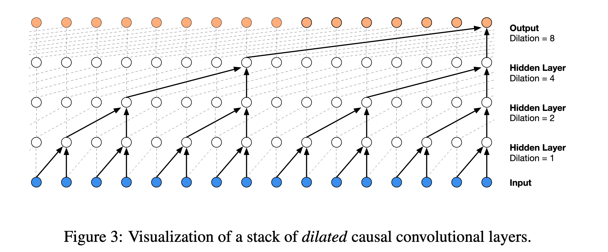
A wavenet is a neural network featuring a "dilated causal convolutional layers" architeture. Despite the fancy terminalogy, the nature is very simple: it converts each input sample, which is typically a time-sequence data and has a shape of T, to a output data with shape (V):

1
[B, T] --> (WaveNet) --> [B, V]
  • T: In WaveNet, each input sample of has shape [T] where T is the time dimenstion (sequence length), i.e., each sample is a time sequence data, such as a sequence of words.
  • B: In practice, the input samples are batched during training. So the shape of input data is [B, T] where B is the batch dimenstion (batch size).
  • V: The output of WaveNet is usually expected to be a logit of some probability, such as the probability for the next English character, in which case V=26 since the alphabet of English is 26.

Steps

The forward pass of WaveNet has following steps:

  1. First, we use a embedding layer to create a embedding for each input sample. In the figure above, a embedding is created as a 16-D vector for a sample.

    1
    [B, T] --> [B, T, C] 

    where C is the embedding dimenstion.

  2. After that, use a flatten layer to flatten the embedding dimenstions by half. Thus, a 16-D embedding becomes a 8-D embedding.

    1
    [B, T, C] --> [B, T//2, C*2] 
  3. Do some other stuff, like applying batch norm and linear layers.

    1
    [B, T//2, C*2] --> [B, T//2, H]

    where H is the hidden dimenstion in the MLP/linear layer.

  4. Repeat step 2-3 until the embedding dimenstion becomes 1. Then we sequeeze out this dimenstion and get the final result.

    1
    [B, T, C] --> [B, T//2, H] --> [B, T//4, H] --> ... --> [B, H]
  5. At last, we apply a linear layer to align with the output shape.

    1
    [B, H] --> [B, V]

Code

Note: Some APIs and requirements are ommited. For details, please refer to my full implementation.

The code is quite compact, we just stack layers together. Note that in the previous figure we have 4 hidden layers converting the time dimenstion as 16 --> 8 --> 4 --> 2 --> 1, whereas in this code implementation, we only have 3 4 hidden layer, and the input time dimenstion is 8, instead of 16, i.e., 8 --> 4 --> 2 --> 1.

1
2
3
4
5
6
7
8
9
10
11
12
13
14
15
16
17
18
19
20
21
22
23
24
25
26
27
28
29
30
31
32
33
# hierarchical network
n_embd = 24 # the dimensionality of the character embedding vectors
n_hidden = 128 # the number of neurons in the hidden layer of the MLP
model = Sequential([
Embedding(vocab_size, n_embd), # [B, T] --> [B, T, C]. [32, 8] --> [32, 8, 24]

FlattenConsecutive(2), # [B, T, C] --> [B, T//2, C*2]. [32, 8, 24] --> [32, 4, 48]
Linear(n_embd * 2, n_hidden, bias=False), # [B, T//2, C*2] --> [B, T//2, H]. [32, 4, 48] --> [32, 4, 128]
BatchNorm1d(n_hidden), # [B, T//2, H] --> [B, T//2, H]. [32, 4, 128] --> [32, 4, 128]
Tanh(), # [B, T//2, H] --> [B, T//2, H]. [32, 4, 128] --> [32, 4, 128]

FlattenConsecutive(2), # [B, T//2, H] --> [B, T//4, H*2]. [32, 4, 128] --> [32, 2, 256]
Linear(n_hidden*2, n_hidden, bias=False), # [B, T//4, H*2] --> [B, T//4, H]. [32, 2, 256] --> [32, 2, 128]
BatchNorm1d(n_hidden),
Tanh(),

FlattenConsecutive(2), # [B, T//4, H] --> [B, T//8, H*2] --> [B, H*2]. [32, 2, 128] --> [32, 1, 256] --> [32, 256]
Linear(n_hidden*2, n_hidden, bias=False), # [B, H*2] --> [B, H]. [32, 256] --> [32, 128]
BatchNorm1d(n_hidden),
Tanh(),

Linear(n_hidden, vocab_size), # [B, H] --> [B, V]. [32, 128] --> [32, 27]

])

# parameter init
with torch.no_grad():
model.layers[-1].weight *= 0.1 # last layer make less confident

parameters = model.parameters()
print(sum(p.nelement() for p in parameters)) # number of parameters in total
for p in parameters:
p.requires_grad = True

The WaveNet architecture is:

1
2
3
4
5
6
7
model = Sequential([
Embedding(vocab_size, n_embd),
FlattenConsecutive(2), Linear(n_embd * 2, n_hidden, bias=False), BatchNorm1d(n_hidden), Tanh(),
FlattenConsecutive(2), Linear(n_hidden*2, n_hidden, bias=False), BatchNorm1d(n_hidden), Tanh(),
Linear(n_hidden, vocab_size),
])

The implementation of each class of layers can be seen in Appendix.

Training

Now we train the WaveNet. We apply following designes:

  1. The maximun steps is set to 200000.

  2. Loss fnction is set to cross entropy.

  3. We use SGD as the optimizer and leverage learning rate decay, i.e.,

    1
    2
    3
    lr = 0.1 if i < 150000 else 0.01 # step learning rate decay
    for p in parameters:
    p.data += -lr * p.grad
1
2
3
4
5
6
7
8
9
10
11
12
13
14
15
16
17
18
19
20
21
22
23
24
25
26
27
28
29
# same optimization as last time
max_steps = 200000
batch_size = 32
lossi = [] # To store the losses during training

for i in range(max_steps):
# minibatch construct
ix = torch.randint(0, Xtr.shape[0], (batch_size,)) # A batch of indices. Each index is a random integer ranging from 0 to Xtr.shape[0]-1.

Xb, Yb = Xtr[ix], Ytr[ix] # batch X,Y. # Each single sample is a context (length=8)

# forward pass
logits = model(Xb) # Each context (8-D vector) is converted to a 27-D vector.
loss = F.cross_entropy(logits, Yb) # loss function

# backward pass
for p in parameters:
p.grad = None
loss.backward()

# update: simple SGD
lr = 0.1 if i < 150000 else 0.01 # step learning rate decay
for p in parameters:
p.data += -lr * p.grad

# track stats
if i % 10000 == 0: # print every once in a while
print(f'{i:7d}/{max_steps:7d}: {loss.item():.4f}')
lossi.append(loss.log10().item())

We can visualize the loss during training:

1
plt.plot(torch.tensor(lossi).view(-1, 1000).mean(1))

Inferrence

We can do inferrence, which means we can sample from the WaveNet (preciesely, from the probability distribution output by the WaveNet).

1
2
3
4
5
6
7
8
9
10
11
12
13
14
15
16
17
18
19
# sample from the model
for _ in range(20):

out = []
context = [0] * block_size # initialize with all ...
while True:
# forward pass the neural net
logits = model(torch.tensor([context]))
probs = F.softmax(logits, dim=1)
# sample from the distribution
ix = torch.multinomial(probs, num_samples=1).item()
# shift the context window and track the samples
context = context[1:] + [ix]
out.append(ix)
# if we sample the special '.' token, break
if ix == 0:
break

print(''.join(itos[i] for i in out)) # decode and print the generated word

Appendix

Linear

The linear layer used in this article is:

1
2
3
4
5
6
7
8
9
10
11
12
13
14
15
16
17
18
class Linear:
'''
Each single sample `x` is a row vector of shape (fan_in). The weight matrix `W` is of shape (fan_in, fan_out).
Thus, the output of `x @ W` is a row vector of shape (fan_out).
In practice, the samples are batched, so the input have shape (batch_size, fan_in), and the output has shape (batch_size, fan_out).
'''
def __init__(self, fan_in, fan_out, bias=True):
self.weight = torch.randn((fan_in, fan_out)) / fan_in**0.5 # Kaiming init with gain=1
self.bias = torch.zeros(fan_out) if bias else None

def __call__(self, x):
self.out = x @ self.weight
if self.bias is not None:
self.out += self.bias
return self.out

def parameters(self):
return [self.weight] + ([] if self.bias is None else [self.bias])

BatchNorm1d

The BatchNorm1d I used resembles PyTorch's torch.nn.BatchNorm1d (Source).

1
2
3
4
5
6
7
8
9
10
11
12
13
14
15
16
17
18
19
20
21
22
23
24
25
26
27
28
29
30
31
32
33
34
35
36
37
38
39
40
41
class BatchNorm1d:

def __init__(self, dim, eps=1e-5, momentum=0.1):
'''
dim: the feature dimension (i.e., the number of features) of a sample.
'''
self.eps = eps
self.momentum = momentum
self.training = True
# parameters (trained with backprop)
self.gamma = torch.ones(dim)
self.beta = torch.zeros(dim)
# buffers (trained with a running 'momentum update')
self.running_mean = torch.zeros(dim)
self.running_var = torch.ones(dim)

def __call__(self, x):
# calculate the forward pass
if self.training:
if x.ndim == 2: # [B, C], i.e., [batch_size, num_features]
dim = 0 # Batch space: [batch_size]
elif x.ndim == 3: # [B, T, C], i.e., [batch_size, num_sequences, num_features].
dim = (0,1) # Batch space: [batch_size, num_sequences]
xmean = x.mean(dim, keepdim=True) # batch mean. Calculate mean for the whole batch space.
xvar = x.var(dim, keepdim=True) # batch variance. Calculate (unbiased) variance for the whole batch space.
else:
# During inference (i.e., evaluation or testing of the model), you typically process one instance at a time. In this case, we can't compute the unbiased var.
# As a result, we use the running mean and variance to normalize the data.
xmean = self.running_mean
xvar = self.running_var
xhat = (x - xmean) / torch.sqrt(xvar + self.eps) # normalize to unit variance
self.out = self.gamma * xhat + self.beta
# update the buffers
if self.training:
with torch.no_grad():
self.running_mean = (1 - self.momentum) * self.running_mean + self.momentum * xmean
self.running_var = (1 - self.momentum) * self.running_var + self.momentum * xvar
return self.out

def parameters(self):
return [self.gamma, self.beta]

Tanh

The Sequential class I used resembles PyTorch's torch.nn.Tanh (Source).

1
2
3
4
5
6
class Tanh:
def __call__(self, x):
self.out = torch.tanh(x)
return self.out
def parameters(self):
return []

Embedding

The Embedding class I used resembles PyTorch's torch.nn.Embedding (Source).

This module is often used to store word embeddings and retrieve them using indices. The input to the module is a list of indices, and the output is the corresponding word embeddings.

1
2
3
4
5
6
7
8
9
10
11
12
13
14
15
16
class Embedding:
'''
A simple lookup table that stores embeddings of a fixed dictionary and size.
Each input sample is a tensor of indices of shape (batch_size, num_features) and the output is the corresponding embeddings of shape (batch_size, num_features, embedding_dim).
'''
def __init__(self, num_embeddings, embedding_dim):
self.weight = torch.randn((num_embeddings, embedding_dim))

def __call__(self, IX):
# print(f"IX shape: {IX.shape}")
# print(f"weight shape: {self.weight.shape}")
self.out = self.weight[IX]
return self.out

def parameters(self):
return [self.weight]

Basic usage:

1
2
3
4
5
ix = torch.randint(0, vocab_size, (3,)) # Get a batch of 3 samples. Each sample is a single integer index ranging from 0 to vocab_size-1, used to select one feature in the embedding matrix.
ix.shape
f = Embedding(vocab_size, n_embd)
y = f(ix)
y.shape

FlattenConsecutive

The FlattenConsecutive class I used is similar to torch.nn.Flatten (Source).

It assumes that the input has shape [B, T, C], representing batch size, sequence length and channel number.

It accepts a flatten factor during initialization and will flatten the the sequence dimenstion (T) of each input according to that factor.

If the flattened sequence dimension becomes 1, it will be sequeezed out.

1
2
3
4
5
6
7
8
9
10
11
12
13
14
15
16
17
class FlattenConsecutive:
'''
To do flattening betwwen layers.
'''
def __init__(self, n):
self.n = n

def __call__(self, x):
B, T, C = x.shape
x = x.view(B, T//self.n, C*self.n)
if x.shape[1] == 1: # If we have only one sequence, squeeze it out. (B, T=1, C) --> (B, C)
x = x.squeeze(1)
self.out = x
return self.out

def parameters(self):
return []

Sequential

The Sequential class I used resembles PyTorch's torch.nn.Sequential (Source). It is a sequential container for layers.

1
2
3
4
5
6
7
8
9
10
11
12
13
14
class Sequential:

def __init__(self, layers):
self.layers = layers

def __call__(self, x):
for layer in self.layers:
x = layer(x)
self.out = x
return self.out

def parameters(self):
# get parameters of all layers and stretch them out into one list
return [p for layer in self.layers for p in layer.parameters()]