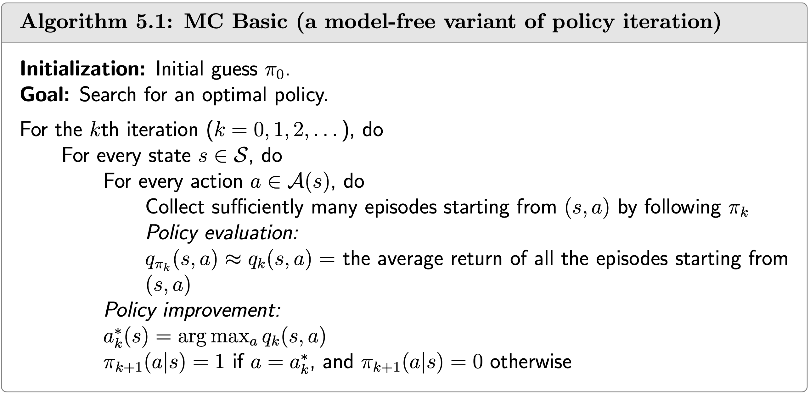
The MC Basic Algorithm
- Shiyu Zhao. Chapter 5: Monte Carlo Methods. Mathematical Foundations of Reinforcement Learning.
- –> Youtube: MC Basic
Motivation
Recalling that the policy iteration algorithm has two steps in each iteration:
- Policy evaluation(PE): \(v_{\pi_k}=r_{\pi_k}+\gamma P_{\pi_k} v_{\pi_k}\).
- Policy improvement(PI): \(\pi_{k+1}=\arg \max _\pi\left(r_\pi+\gamma P_\pi v_{\pi_k}\right)\).
The PE step is calculated through solving the Bellman equation.
The elementwise form of the (PI) step is: \[ \begin{aligned} \pi_{k+1}(s) & =\arg \max _\pi \sum_a \pi(a \mid s)\left[\sum_r p(r \mid s, a) r+\gamma \sum_{s^{\prime}} p\left(s^{\prime} \mid s, a\right) v_{\pi_k}\left(s^{\prime}\right)\right] \\ & =\arg \max _\pi \sum_a \pi(a \mid s) q_{\pi_k}(s, a), \quad s \in \mathcal{S} \end{aligned} \]
The key is \(q_{\pi_k}(s, a)\)! So how can we compute \(q_{\pi_k}(s, a)\)?
Model based case
Since the policy iteration algorithm is a model based algorithm, i.e., the model is given. Recalling that the model (or dynamic) of a MDP is composed of two parts:
- State transition probability: \(p\left(s^{\prime} \mid s, a\right)\).
- Reward probability: \(p(r \mid s, a)\).
Thus, we can calculate \(q_{\pi_k}(s, a)\) via following equation \[ q_{\pi_k}(s, a)=\sum_r p(r \mid s, a) r+\gamma \sum_{s^{\prime}} p\left(s^{\prime} \mid s, a\right) v_{\pi_k}\left(s^{\prime}\right) \] where \(p\left(s^{\prime} \mid s, a\right)\) and \(p(r \mid s, a)\) are given, and every \(v_{\pi_k}\left(s^{\prime}\right)\) is calculated in the PE step.
Model free case
But what if we don’t know the model, i.e., we want to convert policy iteration to a model based algorhtm?
Recalling the definition of action value: \[ \begin{equation} \label{eq_def_of_action_value} q_\pi(s, a) \triangleq \mathbb{E}\left[G_t \mid S_t=s, A_t=a\right] \end{equation} \]
We can use expression \(\eqref{eq_def_of_action_value}\) to calculate \(q_{\pi_k}(s, a)\) based on data (samples or experiences).
This is the key idea of MBRL: If we don’t have a model, we estimate one based on data (or experience).
The procedure of Monte Carlo estimation of action values
- Starting from \((s, a)\), following policy \(\pi_k\), generate an episode.
- The return of this episode is \(g(s, a)\)
- \(g(s, a)\) is a sample of \(G_t\) in \[ q_{\pi_k}(s, a)=\mathbb{E}\left[G_t \mid S_t=s, A_t=a\right] \] Suppose we have a set of episodes and hence \(\left\{g^{(j)}(s, a)\right\}\). Then, \[ q_{\pi_k}(s, a)=\mathbb{E}\left[G_t \mid S_t=s, A_t=a\right] \approx \frac{1}{N} \sum_{i=1}^N g^{(i)}(s, a) \]
The idea of estimate the mean based on data is called Monte Carlo estimation. This is why our method is called “MC (Monte Carlo)” Basic.
The MC Basic algorithm
The MC Basic algorithm is exactly the same as the policy iteration algorithm except: In policy evaluation (PI), we don’t solve \(v_{\pi_k}(s)\), instead we estimate \(q_{\pi_k}(s, a)\) directly.
Question: why we don’t compute \(v_{\pi_k}(s)\)?
Answer: If we calculate the state value in PE, in PI step we still need to calculate activion value. So we can directly calculate activion value in PE.
The MC Basic algorithm is convergent since the policy iteration algorithm (MC Basic is just a variant of it) is convergent.
However, the MC Basic algorithm is not practical due its low data efficiency (we need to calculate \(N\) episodes for every \(q_{\pi_k}(s, a)\)).
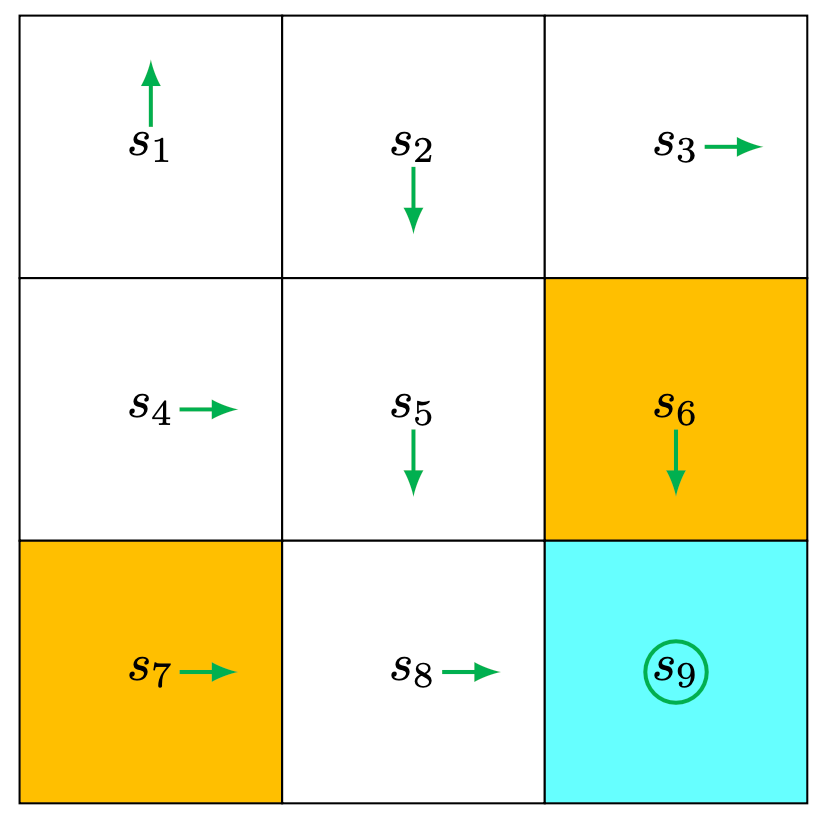
Example
An initial policy is shown in the figure (as you can see, it’s a deterministic policy). Use MC Basic to find the optimal policy. The env setting is: \[
r_{\text {boundary }}=-1, r_{\text {forbidden }}=-1, r_{\text {target }}=1, \gamma=0.9 .
\] 
Outline: given the current policy \(\pi_k\), in each iteration: 1. policy evaluation: calculate \(q_{\pi_k}(s, a)\). Sicne there’re 9 states and 5 actions. We need to calculate 45 state-action pairs. 2. policy improvement: select the greedy action
\[ a^*(s)=\arg \max _{a_i} q_{\pi_k}(s, a) \]
For each state-action pair, we need to roll out \(N\) episodes to estimate the action value. However, since it’s a deterministic policy, we only need to rollout 1 step.
For space limitation, we only illustrate for the part of action value for \(s_1\) in the first iteration.
Step 1: policy evaluation
- Starting from \(\left(s_1, a_1\right)\), the episode is \(s_1 \xrightarrow{a_1} s_1 \xrightarrow{a_1} s_1 \xrightarrow{a_1} \ldots\) Hence, the action value is
\[ q_{\pi_0}\left(s_1, a_1\right)=-1+\gamma(-1)+\gamma^2(-1)+\ldots \]
- Starting from \(\left(s_1, a_2\right)\), the episode is \(s_1 \xrightarrow{a_2} s_2 \xrightarrow{a_3} s_5 \xrightarrow{a_3} \ldots\) Hence, the action value is
\[ q_{\pi_0}\left(s_1, a_2\right)=0+\gamma 0+\gamma^2 0+\gamma^3(1)+\gamma^4(1)+\ldots \]
- Starting from \(\left(s_1, a_3\right)\), the episode is \(s_1 \xrightarrow{a_3} s_4 \xrightarrow{a_2} s_5 \xrightarrow{a_3} \ldots\) Hence, the action value is
\[ q_{\pi_0}\left(s_1, a_3\right)=0+\gamma 0+\gamma^2 0+\gamma^3(1)+\gamma^4(1)+\ldots \]
- Starting from \(\left(s_1, a_4\right)\), the episode is \(s_1 \xrightarrow{a_4} s_1 \xrightarrow{a_1} s_1 \xrightarrow{a_1} \ldots\) Hence, the action value is
\[ q_{\pi_0}\left(s_1, a_4\right)=-1+\gamma(-1)+\gamma^2(-1)+\ldots \] 5. Starting from \(\left(s_1, a_5\right)\), the episode is \(s_1 \xrightarrow{a_5} s_1 \xrightarrow{a_1} s_1 \xrightarrow{a_1} \ldots\) Hence, the action value is
\[ q_{\pi_0}\left(s_1, a_5\right)=0+\gamma(-1)+\gamma^2(-1)+\ldots \]
Step2: policy improvement
By observing the action values, we see that \[ q_{\pi_0}\left(s_1, a_2\right)=q_{\pi_0}\left(s_1, a_3\right) \] are the maximum.
As a result, the policy can be improved as \[ \pi_1\left(a_2 \mid s_1\right)=1 \text { or } \pi_1\left(a_3 \mid s_1\right)=1 \text {. } \]
In either way, the new policy for \(s_1\) becomes optimal.
Drawback
We can see the drawback of MC Basic algorithm: for any episode, we must calculate the discounted return \(G_t\) of it, i.e., we must wait until an episode has been completed.
How long should the episode length be?
As can been seen in previous, in each episode the reward is calculated through a process like
Starting from \(\left(s_1, a_1\right)\), the episode is \(s_1 \xrightarrow{a_1} s_1 \xrightarrow{a_1} s_1 \xrightarrow{a_1} \ldots\) Hence, the action value is \[ q_{\pi_0}\left(s_1, a_1\right)=-1+\gamma(-1)+\gamma^2(-1)+\ldots \]
In practice, we use the finite episode length. We have shown that the state value obtained via an iteration process \[ v_{\pi_k}^{(j+1)}=r_{\pi_k}+\gamma P_{\pi_k} v_{\pi_k}^{(j)}, \quad j=0,1,2, \ldots \] is ensured to have \(v_{\pi_k}^{(j)} \rightarrow v_{\pi_k}\) as \(j \rightarrow \infty\) (–>See the proof), from any initial guess \(v_{\pi_k}^{(0)}\).
However, what if the finite episode length is too small and \(v_{\pi_k}^{(j)}\) does not converge to \(v_{\pi_k}\). In this case, the action value won’t be correct, and the premise of the reasoning falls apart.
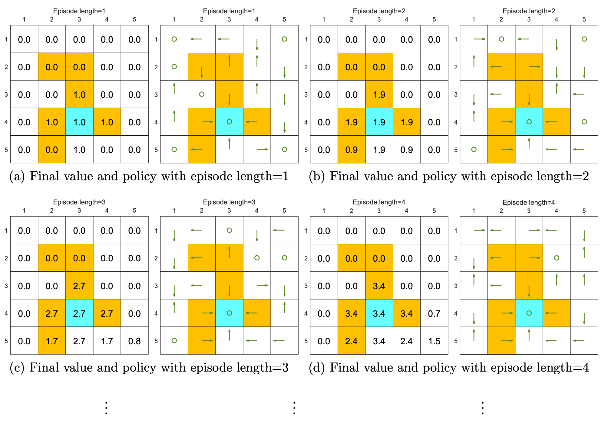
We can see from the following figures that, the episode length greatly impacts the final optimal poli- cies.
When the length of each episode is too short, neither the policy nor the value estimate is optimal (see Figures 5.4(a)-(d)). In the extreme case where the episode length is one, only the states that are adjacent to the target have nonzero values, and all the other states have zero values since each episode is too short to reach the target or get positive rewards (see Figure 5.4(a)).
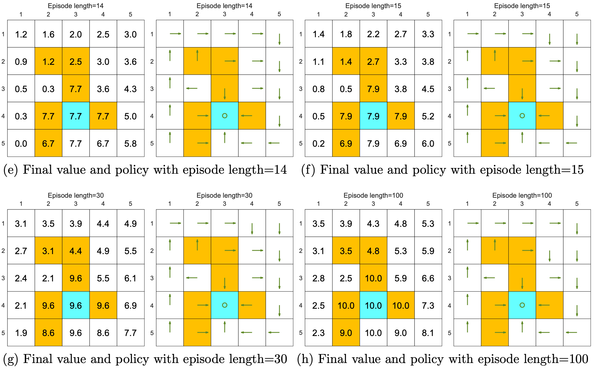
As the episode length increases, the policy and value estimates gradually approach the optimal ones (see Fig- ure 5.4(h)).
While the above analysis suggests that each episode must be sufficiently long, the episodes are not necessarily infinitely long. As shown in Figure 5.4(g), when the length is 30, the algorithm can find an optimal policy, although the value estimate is not yet optimal.
The above analysis is related to an important reward design problem, sparse reward, which refers to the scenario in which no positive rewards can be obtained unless the target is reached. The sparse reward setting requires long episodes that can reach the target. This requirement is challenging to satisfy when the state space is large. As a result, the sparse reward problem downgrades the learning efficiency.