Univariate Gaussian Distributions

Posted on 2024-01-20 Edited on 2024-09-17 In Mathematics Views:

Sources:

The Normal/Gaussian Random Variable

Notations

In this article we'll use following notations interchangeably.

The PDF¹ $f_X(x)$ is often denoted as $p_X(x), $ $f_X\left(x ; \mu, \sigma^2\right)$ or $p_X\left(x ; \mu, \sigma^2\right)$. We sometimes also omit the subscript $X$ so that we can write things like $f(x:\mu,\sigma^2)$.
A normal distribution is also called a Gaussian distribution.
Since a normal distribution is fully determined by its mean $\mu$ and variance $\sigma^2$ (or standard deviation $\sigma$), we often denote a normal distribution as \[ \mathcal{N}(\mu,\sigma^2) . \] A random variable, say $X$, having this distribution is denoted as \[ X \sim \mathcal{N}(\mu,\sigma^2) . \]
The notation $X \sim \mathcal{N}(\mu,\sigma^2)$ can also be written as $X \sim \mathcal{N}(x:\mu_x,\sigma_x^2)$.
We usually call a random variable $X$ having the normal distribution as:
1. normal (or Gaussian) $X$
2. normal (or Gaussian) variable $X$
3. normal (or Gaussian) random variable $X$
For a random variable having standard normal distribution, we often use the notation $Z$, i.e., $Z \sim \mathcal{N}(0, I)$. Meanwhile, $Z$ is also called:
1. standard normal (or Gaussian) $Z$
2. standard normal (or Gaussian) variable $Z$
3. standard normal (or Gaussian) random variable $Z$
We use $\exp(\cdots)$ to represent the where $\exp$ denotes the exponential function $e^{(\cdots)}$.

Definition

In statistics, a normal distribution or Gaussian distribution is a type of continuous probability distribution for a real-valued random variable.

We use $X \sim \mathcal N\left(\mu, \sigma^2\right)$ to denote that a real-valued random variable $X$ follows the Gaussian distribution with mean=$\mu$ and standard deviation=$\sigma$.

The PDF for $X$ is:

\[ f_X(x)=\frac{1}{\sigma \sqrt{2 \pi}} \exp({-\frac{1}{2}\left(\frac{x-\mu}{\sigma}\right)^2}) \]

By definition,

$\mu$ is the mean or expectation of the distribution \[ \mathbb E[X] = \mu , \]
$\sigma^2$ is the variance of the distribution \[ \mathrm{Var}(X) = \sigma^2 . \]

You can think of the coefficient in front, $\frac{1}{\sqrt{2 \pi} \sigma}$, as simply a constant "normalization factor" used to ensure that \[ \frac{1}{\sqrt{2 \pi} \sigma} \int_{-\infty}^{\infty} \exp \left(-\frac{1}{2 \sigma^2}(x-\mu)^2\right)=1 . \]

Notice the $x$ in the exponent of the PDF function. When $x$ is equal to the mean $(\mu)$ then $\mathrm{e}$ is raised to the power of 0 and the PDF is maximized.

Explanation

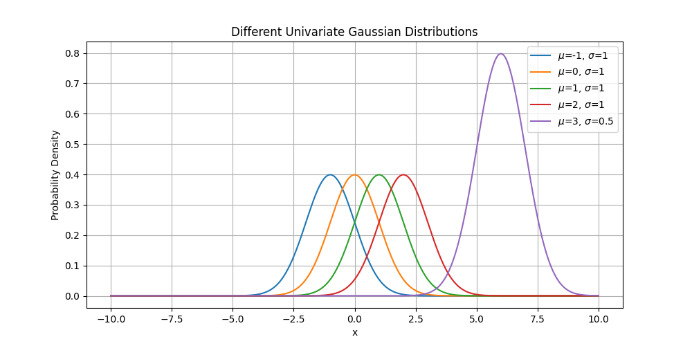
$\sigma$ describes the spread of the data points around the mean.

$\mu$ defines the central location of the Gaussian distribution.

Code

import torch
def calculate_univariate_gaussian_distribution(x, mu, sigma):
    leading_coefficient = 1 / (sigma * torch.sqrt(torch.tensor(2 * torch.pi)))
    parameter_of_exp_function = -0.5 * (x - mu / sigma) ** 2
    return leading_coefficient * torch.exp(parameter_of_exp_function)

Standard Normal

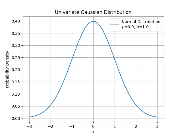
A normal distribution $\mathcal{N}(\mu,\sigma^2)$ is standard if $\mu = 0$ and $\sigma^2 = 1$.

The random variable that follows a normal distribution is often denoted as \[ Z \sim \mathcal{N}(0,1) . \] $Z$ is called the stanard normal.

Closure properties of the normal distribution

Recall that in general, if $X$ is any random variable (discrete or continuous) with $\mathbb{E}[X]=\mu$ and $\operatorname{Var}(X)=\sigma^2$, and $a, b \in \mathbb{R}$. Then, \[ \begin{aligned} & \mathbb{E}[a X+b]=a \mathbb{E}[X]+b=a \mu+b \\ & \operatorname{Var}(a X+b)=a^2 \operatorname{Var}(X)=a^2 \sigma^2 \end{aligned} \]

Closure of the Normal Under Scale and Shift

If $X \sim \mathcal{N}\left(\mu, \sigma^2\right)$, then $a X+b \sim \mathcal{N}\left(a \mu+b, a^2 \sigma^2\right)$. In particular, \[ \frac{X-\mu}{\sigma} \sim \mathcal{N}(0,1) \]

We will prove this theorem later using Moment Generating Functions! This is really amazing the mean and variance are no surprise. The fact that scaling and shifting a Normal random variable results in another Normal random variable is very interesting!

Let $X, Y$ be ANY independent random variables (discrete or continuous) with $\mathbb{E}[X]=\mu_X, \mathbb{E}[Y]=\mu_Y$, $\operatorname{Var}(X)=\sigma_X^2, \operatorname{Var}(Y)=\sigma_Y^2$ and $a, b, c \in \mathbb{R}$. Recall, \[ \begin{gathered} \mathbb{E}[a X+b Y+c]=a \mathbb{E}[X]+b \mathbb{E}[Y]+c=a \mu_X+b \mu_Y+c \\ \operatorname{Var}(a X+b Y+c)=a^2 \operatorname{Var}(X)+b^2 \operatorname{Var}(Y)=a^2 \sigma_X^2+b^2 \sigma_Y^2 \end{gathered} \]

Closure of the Normal Under Addition

If $X \sim \mathcal{N}\left(\mu_X, \sigma_X^2\right)$ and $Y \sim \mathcal{N}\left(\mu_Y, \sigma_Y^2\right)$ (both independent normal random variables), then \[ a X+b Y+c \sim \mathcal{N}\left(a \mu_X+b \mu_Y+c, a^2 \sigma_X^2+b^2 \sigma_Y^2\right) \]

Again, this is really amazing. The mean and variance aren't a surprise again, but the fact that adding two independent Normals results in another Normal distribution is not trivial, and we will prove this later as well!

Probability density function↩︎