Variational Autoencoders

Sources:

1. VAE paper
2. Mathematics Behind Variational AutoEncoders
3. Variational autoencoders by Matthew N. Bernstein
4. From Autoencoder to Beta-VAE
5. Stanford CS 228: The variational auto-encoder

Link: My VAE implementation on Github

Notations

Symbol	Mean
\(\mathcal{D}\)	The dataset, \(\mathcal{D} = \left\{ \mathbf{x}^{(1)}, \mathbf{x}^{(2)}, \ldots, \mathbf{x}^{(n)} \right\}\), contains \(n\) data samples; \(|\mathcal{D}| = n\).
\(\mathbf{x}^{(i)}\)	Each data point is a vector of \(d\) dimensions, \(\mathbf{x}^{(i)} = \left[ x_1^{(i)}, x_2^{(i)}, \ldots, x_d^{(i)} \right]\).
\(\mathbf{x}\)	One data sample from the dataset, \(\mathbf{x} \in \mathcal{D}\).
\(\mathbf{x}^{\prime}\)	The reconstructed version of \(\mathbf{x}\).
\(\tilde{\mathbf{x}}\)	The corrupted version of \(\mathbf{x}\).
\(\mathbf{z}\)	The compressed code learned in the bottleneck layer.
\(a_j^{(l)}\)	The activation function for the \(j\)-th neuron in the \(l\)-th hidden layer.
\(g_\phi(\cdot)\)	The encoding function parameterized by \(\phi\).
\(f_\theta(\cdot)\)	The decoding function parameterized by \(\theta\).
\(q_\phi(\mathbf{z} \mid \mathbf{x})\)	Estimated posterior probability function, also known as probabilistic encoder.
\(p_\theta(\mathbf{x} \mid \mathbf{z})\)	Likelihood of generating true data sample given the latent code, also known as probabilistic decoder. d

Autoencoders

Autoencoder is a neural network designed to learn an identity function in an unsupervised way to reconstruct the original input while compressing the data in the process so as to discover a more efficient and compressed representation. The idea was originated in the 1980s, and later promoted by the seminal paper by Hinton & Salakhutdinov, 2006.

It consists of two networks:

• Encoder network: It translates the original high-dimension input into the latent low-dimensional code. The input size is larger than the output size.
• Decoder network: The decoder network recovers the data from the code, likely with larger and larger output layers.

Figure 1

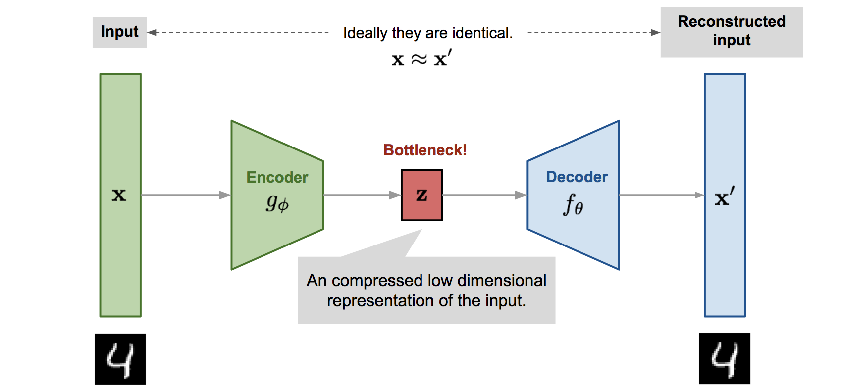
The encoder network essentially accomplishes the dimensionality reduction, just like how we would use Principal Component Analysis (PCA) or Matrix Factorization (MF) for

The model contains:

1. an encoder function \(g(.)\) parameterized by \(\phi\) and
2. a decoder function \(f(.)\) parameterized by \(\theta\).

The low-dimensional code learned for input \(\mathbf{x}\) in the bottleneck layer is \(\mathbf{z}=g_\phi(\mathbf{x})\) and the reconstructed input is \(\mathbf{x}^{\prime}=f_\theta\left(g_\phi(\mathbf{x})\right)\).

The parameters \((\theta, \phi)\) are learned together to output a reconstructed data sample same as the original input, \(\mathbf{x} \approx f_\theta\left(g_\phi(\mathbf{x})\right)\), or in other words, to learn an identity function.

There are various metrics to quantify the difference between two vectors, such as cross entropy when the activation function is sigmoid, or as simple as MSE loss: \[ L_{\mathrm{AE}}(\theta, \phi)=\frac{1}{n} \sum_{i=1}^n\left(\mathbf{x}^{(i)}-f_\theta\left(g_\phi\left(\mathbf{x}^{(i)}\right)\right)\right)^2 \]

VAE: Variational Autoencoder

The idea of Variational Autoencoder (Kingma & Welling, 2014), short for VAE, is actually less similar to all the autoencoder models above, but deeply rooted in the methods of variational bayesian and graphical model.

Let's consider some dataset consisting of \(\mathrm{N}\) i.i.d. samples of a random variable \(\mathbf{x}\) (either scalar or vector) (Q: why iid?). The data are assumed to be generated by some random process, involving an unobserved random variable \(\mathbf{z}\) (i.e. the latent variable).

The generative process has two steps: 1. a value \(\mathbf{z}^{(\mathbf{i})}\) is generated from some prior distribution \(p_{\boldsymbol{\theta}^*}(\mathbf{z})\), 2. a value \(\mathbf{x}^{(\mathbf{i})}\) is generated from some conditional distribution \(p_{\boldsymbol{\theta}^*}(\mathbf{x} \mid \mathbf{z} = \mathbf{z}^{(\mathbf{i})})\) dependent on \(\mathbf{z}^{(\mathbf{i})}\),

We assume that the prior \(p_{\boldsymbol{\theta}^*}(\mathbf{z})\) and likelihood \(p_{\boldsymbol{\theta}^*}(\mathbf{x} \mid \mathbf{z})\) come from parametric families of distributions \(p_{\boldsymbol{\theta}}(\mathbf{z})\) and \(p_{\boldsymbol{\theta}}(\mathbf{x} \mid \mathbf{z})\), and that their PDFs are differentiable almost almost everywhere w.r.t. both \(θ\) and \(\mathbf{z}\).

(Q: Why we assume they both controled by \(\theta\)?)

The variational method

We are interested in \(p(\mathbf{z} \mid \mathbf{x} = \mathbf{x}^{(i)})\), the posterior inference of the latent variable \(\mathbf{z}\) given an observed value \(\mathbf{x}\) for a choice of parameters \(\theta\). It is useful for representation learning.

We use the variational method to calculate it. The process is:

$$ \[\begin{aligned} p_\theta\left(\mathbf{z} \mid \mathbf{x} = \mathbf{x}^{(i)}\right) & = \frac{p_\theta\left(\mathbf{z}, \mathbf{x} = \mathbf{x}^{(i)}\right)}{p_\theta\left(\mathbf{x} = \mathbf{x}^{(i)}\right)} \\ & = \frac { \textcolor{purple} {p_\theta\left(\mathbf{x}=\mathbf{x}^{(i)} \mid \mathbf{z}\right) p_\theta\left(\mathbf{z}\right)} } { \int_{\mathbf{z}^{(i)}} p_\theta \left(\mathbf{x}=\mathbf{x}^{(i)} \mid \mathbf{z}=\mathbf{z}^{(i)}\right) p_\theta\left(\mathbf{z}=\mathbf{z}^{(i)}\right) d \mathbf{z}^{(i)} } \end{aligned}\]

$$

Suppose that we have a choice for parameters \(\theta\), thus both the specification of the prior distribution \(\textcolor{purple} {p_\theta(\mathbf{z})}\) and the likelihood \(\textcolor{purple} {p_\theta\left(\mathbf{x} =\mathbf{x}^{(\mathbf{i})} \mid \mathbf{z} \right)}\) defined by the generative process would be known.

Therefore theoretically, the posterior \(p_\theta\left(\mathbf{z} \mid \mathbf{x} = \mathbf{x}^{(\mathbf{i})} \right)\) can be calculated after evaluating the integral in the denominator, which involves enumerating all the possible values the unobservable variable \(\mathrm{z}\) may have.

However without any simplifying assumptions on \(p\left(\mathbf{z} \mid \mathbf{x}\mathbf{x}^{(\mathbf{i})} ; \theta\right)\) or \(p(\mathbf{z} ; \theta)\), the integral is intractable, as it is very expensive to check all the possible values of \(\mathbf{z}\) and sum them up.

To solve this, the variational method introduces a so-called recognition model \(q_\phi(\mathbf{z} \mid \mathbf{x} = \mathbf{x}^{(i)})\), parameterized by \(\phi\), as an approximation to the true posterior \(p_\theta\left(\mathbf{z} \mid \mathbf{x} = \mathbf{x}^{(i)}\right)\).

Assumptions

In practice, we will always assume the encoder output distribution \(q_\phi\left(\mathbf{z} \mid \mathbf{x} = \mathbf{x}^{(i)}\right)\) to be a multivariate gaussian: \[ \mathbf{z} \sim q_\phi\left(\mathbf{z} \mid \mathbf{x} = \mathbf{x}^{(i)}\right) = \mathcal{N}\left(\boldsymbol{\mu}^{(i)}, (\boldsymbol{\sigma}^{(i)})^2 \boldsymbol{I}\right) . \]

In practice, we will always assume the prior distribution \(p_\theta(z)\) to be a multivariate standard gaussian: \[ \mathbf{z} \sim p_\phi\left(\mathbf{z}\right)=\mathcal{N}\left(\boldsymbol{0}, \boldsymbol{I}\right) . \]

The loss function: negative ELBO

The estimated posterior \(q_\phi(\mathbf{z} \mid \mathbf{x})\) should be very close to the real one \(p_\theta(\mathbf{z} \mid \mathbf{x})\). We want to reduce the Kullback-Leibler divergence of between these two distributions: \[ \begin{aligned} D_{\mathrm{KL}}\left(q_\phi\left(\mathbf{z} \mid \mathbf{x} = \mathbf{x}^{(i)}\right) \| p_\theta\left(\mathbf{z} \mid \mathbf{x} = \mathbf{x}^{(i)}\right)\right) & = \int_{\mathbf{z}} q_\phi\left(\mathbf{z} \mid \mathbf{x} = \mathbf{x}^{(i)}\right) \log \frac{q_\phi\left(\mathbf{z} \mid \mathbf{x} = \mathbf{x}^{(i)}\right)}{p_\theta\left(\mathbf{z} \mid \mathbf{x} = \mathbf{x}^{(i)}\right)} d \mathbf{z} \\ & = \mathbb{E}_q\left[\log q_\phi\left(\mathbf{z} \mid \mathbf{x} = \mathbf{x}^{(i)}\right)\right] - \mathbb{E}_q\left[\log p_\theta\left(\mathbf{z} \mid \mathbf{x} = \mathbf{x}^{(i)}\right)\right] \\ & = \mathbb{E}_q\left[\log q_\phi\left(\mathbf{z} \mid \mathbf{x} = \mathbf{x}^{(i)}\right)\right] - \mathbb{E}_q\left[\log p_\theta\left(\mathbf{x} = \mathbf{x}^{(i)}, \mathbf{z}\right)\right] + \mathbb{E}_{q_\phi}\left[\log p_\theta\left(\mathbf{x} = \mathbf{x}^{(i)}\right)\right] \\ & = \mathbb{E}_q\left[\log q_\phi\left(\mathbf{z} \mid \mathbf{x} = \mathbf{x}^{(i)}\right)\right] - \mathbb{E}_q\left[\log p_\theta\left(\mathbf{x} = \mathbf{x}^{(i)}, \mathbf{z}\right)\right] + \log p_\theta\left(\mathbf{x} = \mathbf{x}^{(i)}\right) \\ & = -\text{ELBO}_\theta + \textcolor{blue}{\log p_\theta\left(\mathbf{x} = \mathbf{x}^{(i)}\right) } \end{aligned} \]

(\(\mathbb{E}_q\) means \(\mathbb{E}_{q_{\phi}}\))

where ELBO stands for Evidence Lower BOund, which is defind as: \[ \begin{aligned} \mathrm{ELBO} & = -\mathbb{E}_q\left[\log q_\phi\left(\mathbf{z} \mid \mathbf{x} = \mathbf{x}^{(i)}\right)\right] + \mathbb{E}_q\left[\log p_\theta\left(\mathbf{x} = \mathbf{x}^{(i)}, \mathbf{z}\right)\right] \\ & = -\mathbb{E}_q\left[\log q_\phi\left(\mathbf{z} \mid \mathbf{x} = \mathbf{x}^{(i)}\right)\right] + \mathbb{E}_q\left[\log p_\theta\left(\mathbf{z}\right)\right] + \mathbb{E}_q\left[\log p_\theta\left(\mathbf{x} = \mathbf{x}^{(i)} \mid \mathbf{z}\right)\right] \\ & = -D_{\mathrm{KL}}\left(q_\phi\left(\mathbf{z} \mid \mathbf{x} = \mathbf{x}^{(i)}\right) \| p_\theta(\mathbf{z})\right) + \mathbb{E}_q\left[\log p_\theta\left(\mathbf{x} = \mathbf{x}^{(i)} \mid \mathbf{z}\right)\right] \end{aligned} \] Since the term \(\textcolor{blue}{\log p_\theta\left(\mathbf{x} = \mathbf{x}^{(i)}\right) }\) is a constant, it can be ignored during the optimization process. As the result, the loss function is: \[ \begin{aligned} \mathcal{L}\left(\phi, \theta, \mathbf{x}^{(\mathbf{i})}\right) & = - \mathrm{ELBO} \\ & = \textcolor{pink} {D_{\mathrm{KL}}\left(q_\phi\left(\mathbf{z} \mid \mathbf{x} = \mathbf{x}^{(i)}\right) \| p_\theta(\mathbf{z})\right)} - \textcolor{green} {\mathbb{E}_q\left[\log p_\theta\left(\mathbf{x} = \mathbf{x}^{(i)} \mid \mathbf{z}\right)\right] } \end{aligned} \] ## How to compute the loss function

The expectation term

We will use Monte Carlo method to calculate (or, more precisely, approximate) the expectation term, i.e., \[ \textcolor{green} {\mathbb{E}_q\left[\log p_\theta\left(\mathbf{x} = \mathbf{x}^{(i)} \mid \mathbf{z}\right)\right] \approx \frac{1}{L} \sum_{l=1}^L\left[\log p\left(\mathbf{x}^{(i)} \mid \mathbf{z}^{(i l)} ; \theta\right)\right]} \] when \(L\) is very large.

However, in practice, we will set \(L=1\) to calculate the mean \(\textcolor{green} {\mathbb{E}_q\left[\log p_\theta\left(\mathbf{x} = \mathbf{x}^{(i)} \mid \mathbf{z}\right)\right]}\) (Yeah, you are right. We only use one sample to approximate the expectation. That's radiculous! But somehow they just regulated it.)

So that our approximated mean equals \(\textcolor{green} {\log p\left(\mathbf{x}^{(i)} \mid \mathbf{z}\right)}\): \[ \textcolor{green} {\mathbb{E}_q\left[\log p_\theta\left(\mathbf{x} = \mathbf{x}^{(i)} \mid \mathbf{z}\right)\right] \approx \text{(very weird)} \quad \log p\left(\mathbf{x}^{(i)} \mid \mathbf{z}\right)} \]

The KL term

Meanwhile, according to our assumptions (see the previous section), we will always assume \(q_\phi\left(\mathbf{z} \mid \mathbf{x} = \mathbf{x}^{(i)}\right) = \mathcal{N}\left(\boldsymbol{\mu}^{(i)}, (\boldsymbol{\sigma}^{(i)})^2 \boldsymbol{I}\right)\), \(p_\phi\left(\mathbf{z}\right)=\mathcal{N}\left(\boldsymbol{0}, \boldsymbol{I}\right)\). In this particular case, it turns out that the KL-divergence term above can be expressed analytically (See the Appendix to this post): \[ \textcolor{pink} {D_{\mathrm{KL}}\left(q_\phi\left(\mathbf{z} \mid \mathbf{x} = \mathbf{x}^{(i)}\right) \| p_\theta(\mathbf{z})\right)=-\frac{1}{2} \sum_{j=1}^J\left(1+\log \sigma_j^2-\mu_j^2-\sigma_j^2\right)} \]

The result

So that \[ \begin{aligned} \mathcal{L}\left(\phi, \theta, \mathbf{x}^{(\mathbf{i})}\right) & = \textcolor{pink} { \frac{1}{2} \sum_{j=1}^J\left(1+ \log \sigma^2_j-\mu_j^2-\sigma_j^2\right) } - \textcolor{green} {\log p\left(\mathbf{x}^{(i)} \mid \mathbf{z}\right)} . \end{aligned} \]

Why use reversed KL?

Back in the last section, The loss function: negative ELBO, we regulate the loss function to be \(D_{\mathrm{KL}}\left(q_\phi \mid p_\theta\right)\). But why we choose \(D_{\mathrm{KL}}\left(q_\phi \mid p_\theta\right)\) (reversed KL) instead of \(D_{\mathrm{KL}}\left(p_\theta \mid q_\phi\right)\) (forward KL)?

Eric Jang has a great explanation in his post on Bayesian Variational methods. As a quick recap:

Figure 2

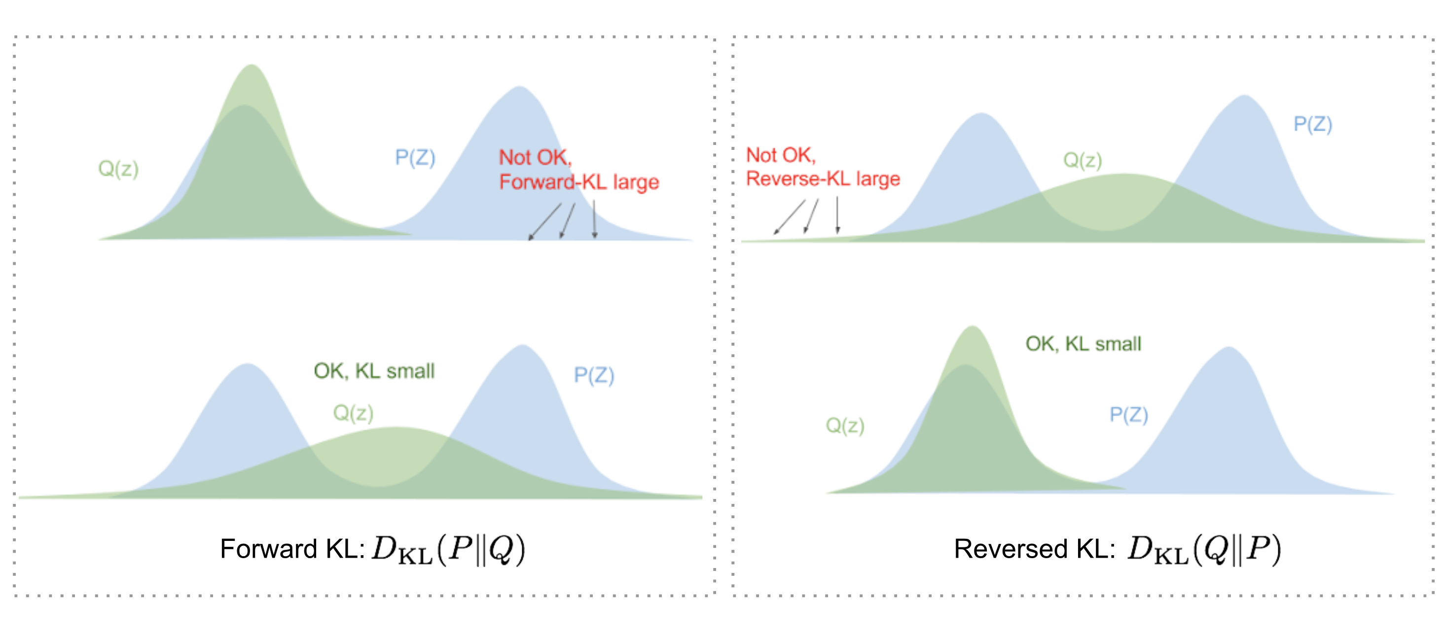
• Forward KL divergence: \(D_{\mathrm{KL}}(P \mid Q)=\mathbb{E}_{z \sim P(z)} \log \frac{P(z)}{Q(z)}\); we have to ensure that \(\mathrm{Q}(\mathrm{z})>0\) wherever \(\mathrm{P}(\mathrm{z})>0\). The optimized variational distribution \(q(z)\) has to cover over the entire \(p(z)\).
• Reversed KL divergence: \(D_{\mathrm{KL}}(Q \mid P)=\mathbb{E}_{z \sim Q(z)} \log \frac{Q(z)}{P(z)}\); minimizing the reversed KL divergence squeezes the \(Q(z)\) under \(P(z)\).

Tricks

Reparameterization trick

Figure 3

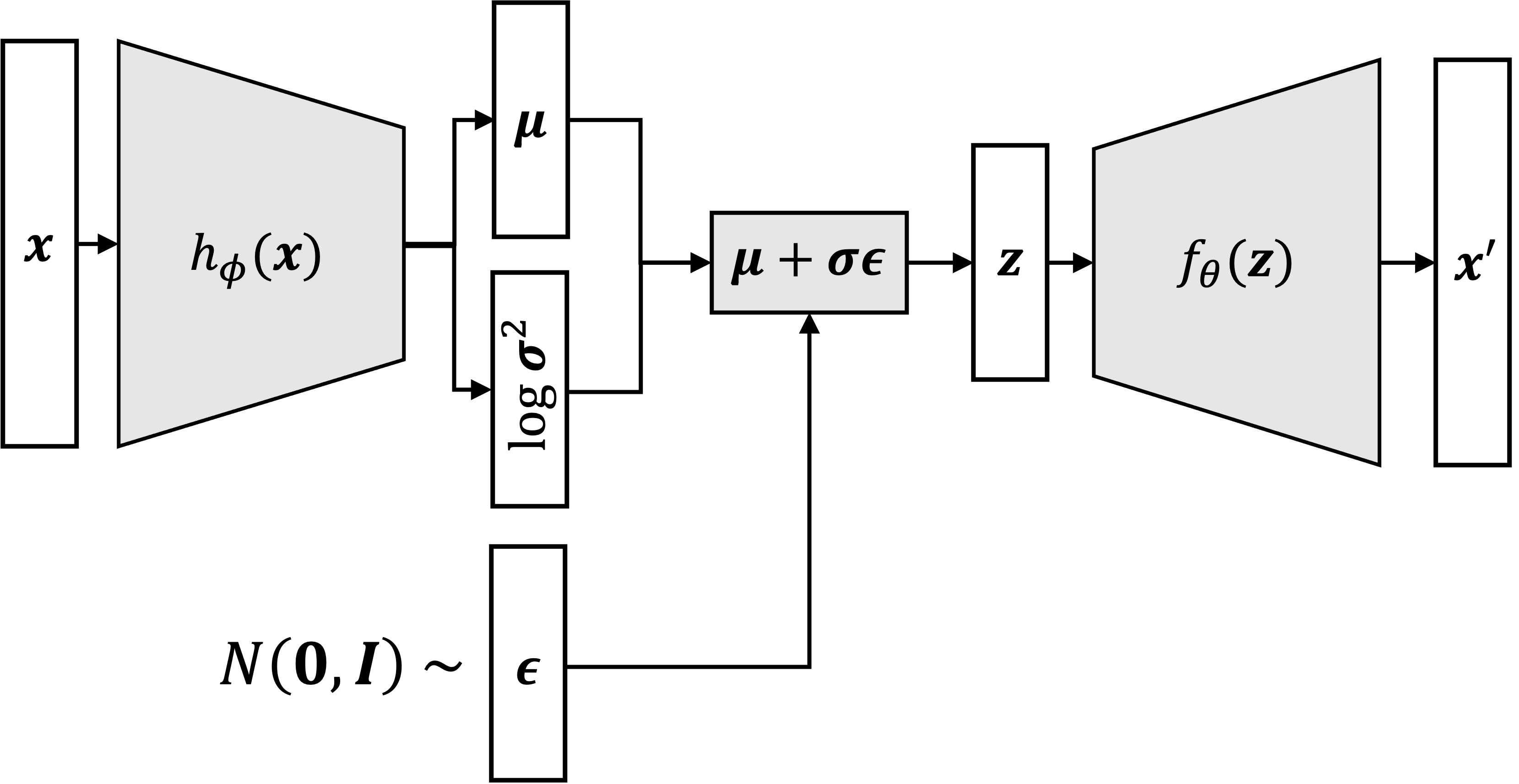
The expectation term in the loss function invokes generating samples from \(\mathbf{z} \sim q_\phi(\mathbf{z} \mid \mathbf{x})\). Sampling is a stochastic process and therefore we cannot backpropagate the gradient.

To make it trainable, the reparameterization trick is introduced: It is often possible to express the random variable \(\mathbf{z}\) as a deterministic variable \(\mathbf{z}=\mathcal{T}_\phi(\mathbf{x}, \boldsymbol{\epsilon})\), where \(\boldsymbol{\epsilon}\) is an auxiliary independent random variable, and the transformation function \(\mathcal{T}_\phi\) parameterized by \(\phi\) converts \(\epsilon\) to \(\mathbf{z}\).

For example, a common choice of the form of \(q_\phi(\mathbf{z} \mid \mathbf{x})\) is a multivariate Gaussian with a diagonal covariance structure: \[ \begin{aligned} & \mathbf{z} \sim q_\phi\left(\mathbf{z} \mid \mathbf{x}^{(i)}\right)=\mathcal{N}\left(\mathbf{z} ; \boldsymbol{\mu}^{(i)}, \boldsymbol{\sigma}^{2(i)} \boldsymbol{I}\right) \quad \text {; Assume it's Gaussian. } \\ & \mathbf{z}=\boldsymbol{\mu}+\boldsymbol{\sigma} \odot \boldsymbol{\epsilon}, \text { where } \boldsymbol{\epsilon} \sim \mathcal{N}(0, \boldsymbol{I}) \quad \text {; Reparameterization trick. } \end{aligned} \] where \(\odot\) refers to element-wise product.

def reparameterization(self, mean, std_var):
	epsilon = torch.randn_like(std_var).to(DEVICE)        
	z = mean + std_var*epsilon                          
	return z

Log var trick

Instead of using variance \(\boldsymbol{\sigma}\), we use the log-variance to allow for positive and negative values: \(\log \left(\boldsymbol{\sigma}^2\right)\)

Why can we do this? \[ \begin{aligned} \log \left(\boldsymbol{\sigma}^2\right) & =2 \cdot \log (\boldsymbol{\sigma}) \\ \log \left(\boldsymbol{\sigma}^2\right) / 2 & =\log (\boldsymbol{\sigma}) \\ \boldsymbol{\sigma} & =e^{\log \left(\boldsymbol{\sigma}^2\right) / 2} \end{aligned} \]

So, when we sample the points, we can do \[ \mathbf{z}=\boldsymbol{\mu}+e^{\log \left(\boldsymbol{\sigma}^2\right) / 2} \odot \boldsymbol{\epsilon} . \]

Model archiecture

VAE model

class Model(nn.Module):
    def __init__(self, Encoder, Decoder):
        super(Model, self).__init__()
        self.Encoder = Encoder
        self.Decoder = Decoder
        
    def reparameterization(self, mean, std_var):
        epsilon = torch.randn_like(std_var).to(DEVICE)        # sampling epsilon. Ensuring that ϵϵ has the same shape as the variance and is on the correct computing device.      
        z = mean + std_var*epsilon                          # reparameterization trick. Calculate z using the provided mean and variance. 
        return z
        
                
    def forward(self, x):
        mean, log_var = self.Encoder(x)
        
        # `log_var` == 2 log σ, where `σ` is the standard deviation of the distribution.
        # So, e^(0.5 * log_var) == e^(log σ) = σ.
        z = self.reparameterization(mean, torch.exp(0.5 * log_var)) # takes exponential function (log var -> var)
        x_hat            = self.Decoder(z)
        
        return x_hat, mean, log_var

Encoder

"""
    A simple implementation of Gaussian MLP Encoder and Decoder
"""

class Encoder(nn.Module):
    
    def __init__(self, input_dim, hidden_dim, latent_dim):
        super(Encoder, self).__init__()

        self.FC_input = nn.Linear(input_dim, hidden_dim)
        self.FC_input2 = nn.Linear(hidden_dim, hidden_dim)
        self.FC_mean  = nn.Linear(hidden_dim, latent_dim)
        self.FC_var   = nn.Linear (hidden_dim, latent_dim)
        
        self.LeakyReLU = nn.LeakyReLU(0.2)
        
        self.training = True
        
    def forward(self, x):
        h_       = self.LeakyReLU(self.FC_input(x))
        h_       = self.LeakyReLU(self.FC_input2(h_))
        mean     = self.FC_mean(h_)
        log_var  = self.FC_var(h_)                     # encoder produces mean and log of variance 
                                                       #             (i.e., parateters of simple tractable normal distribution "q"
        
        return mean, log_var

Decoder

class Decoder(nn.Module):
    def __init__(self, latent_dim, hidden_dim, output_dim):
        super(Decoder, self).__init__()
        self.FC_hidden = nn.Linear(latent_dim, hidden_dim)
        self.FC_hidden2 = nn.Linear(hidden_dim, hidden_dim)
        self.FC_output = nn.Linear(hidden_dim, output_dim)
        
        self.LeakyReLU = nn.LeakyReLU(0.2)
        
    def forward(self, x):
        h     = self.LeakyReLU(self.FC_hidden(x))
        h     = self.LeakyReLU(self.FC_hidden2(h))
        
        x_hat = torch.sigmoid(self.FC_output(h))
        return x_hat
        

Training process

import torch
import torch.nn as nn

import numpy as np

from tqdm import tqdm
from torchvision.utils import save_image, make_grid
from torch.optim import Adam

Hyperparameters:

# Model Hyperparameters

dataset_path = '~/datasets'

cuda = True
DEVICE = torch.device("cuda" if cuda else "cpu")


batch_size = 100

x_dim  = 784
hidden_dim = 400
latent_dim = 200

lr = 1e-3

epochs = 30

Load the dataset

from torchvision.datasets import MNIST
import torchvision.transforms as transforms
from torch.utils.data import DataLoader


mnist_transform = transforms.Compose([
        transforms.ToTensor(),
])

kwargs = {'num_workers': 1, 'pin_memory': True} 

train_dataset = MNIST(dataset_path, transform=mnist_transform, train=True, download=True)
test_dataset  = MNIST(dataset_path, transform=mnist_transform, train=False, download=True)

train_loader = DataLoader(dataset=train_dataset, batch_size=batch_size, shuffle=True, **kwargs)
test_loader  = DataLoader(dataset=test_dataset,  batch_size=batch_size, shuffle=False, **kwargs)

Build the model

encoder = Encoder(input_dim=x_dim, hidden_dim=hidden_dim, latent_dim=latent_dim)
decoder = Decoder(latent_dim=latent_dim, hidden_dim = hidden_dim, output_dim = x_dim)

model = Model(Encoder=encoder, Decoder=decoder).to(DEVICE)
optimizer = Adam(model.parameters(), lr=lr)

Define the loss function

def loss_function(x, x_hat, mean, log_var):
    reproduction_loss = nn.functional.binary_cross_entropy(x_hat, x, reduction='sum')
    KLD      = - 0.5 * torch.sum(1+ log_var - mean.pow(2) - log_var.exp())

    return reproduction_loss + KLD

Start training loop

print("Start training VAE...")
model.train()

for epoch in range(epochs):
    overall_loss = 0
    for batch_idx, (x, _) in enumerate(train_loader):
        x = x.view(batch_size, x_dim)
        x = x.to(DEVICE)

        optimizer.zero_grad()

        x_hat, mean, log_var = model(x)
        loss = loss_function(x, x_hat, mean, log_var)
        
        overall_loss += loss.item()
        
        loss.backward()
        optimizer.step()
        
    print("\tEpoch", epoch + 1, "complete!", "\tAverage Loss: ", overall_loss / (batch_idx*batch_size))
    
print("Finish!!")

Appendix

Derivation of the KL-divergence term when the variational posterior and prior are Gaussian

If we choose the variational distribution \(q_\phi(\boldsymbol{z} \mid \boldsymbol{x})\) to be defined by the following generative process: \[ \begin{aligned} \boldsymbol{\mu} & :=h_\phi^{(1)}(\boldsymbol{x}) \\ \log \boldsymbol{\sigma}^2 & :=h_\phi^{(2)}(\boldsymbol{x}) \\ \boldsymbol{z} & \sim N\left(\boldsymbol{\mu}, \boldsymbol{\sigma}^{\mathbf{2}} \boldsymbol{I}\right) \end{aligned} \] where \(h^{(1)}\) and \(h^{(2)}\) are the two encoding neural networks, and we choose the prior distribution over \(z\) to be a standard normal distribution: \[ p(z):=N(\mathbf{0}, \boldsymbol{I}) \] then the KL-divergence from \(p(z)\) to \(q_\phi(\boldsymbol{z} \mid \boldsymbol{x})\) is given by the following formula: \[ D_{\mathrm{KL}}\left(q_\phi(\boldsymbol{z} \mid \boldsymbol{x}) \| p(z)\right)=-\frac{1}{2} \sum_{j=1}^J\left(1+h_\phi^{(2)}(\boldsymbol{x})_j-\left(h_\phi^{(1)}(\boldsymbol{x})\right)_j^2-\exp \left(h_\phi^2(\boldsymbol{x})_j\right)\right) \] where \(J\) is the dimensionality of \(z\).

Proof:

First, let's re-write the KL-divergence as follows: \[ \begin{align*} D_{\mathrm{KL}}(q_\phi(\boldsymbol{z} \mid \boldsymbol{x}) || p(\boldsymbol{z})) &= \int q_\phi(\boldsymbol{z} \mid \boldsymbol{x}) \log \frac{q_\phi(\boldsymbol{z} \mid \boldsymbol{x})}{ p(\boldsymbol{z}))} \\ &= \int q_\phi(\boldsymbol{z} \mid \boldsymbol{x}) \log q_\phi(\boldsymbol{z} \mid \boldsymbol{x}) \ d\boldsymbol{z} - \int q_\phi(\boldsymbol{z} \mid \boldsymbol{x}) \log p(\boldsymbol{z}) \ d\boldsymbol{z}\end{align*} \]

First, let's compute the first term, \(\int q_\phi(\boldsymbol{z} \mid \boldsymbol{x}) \log q_\phi(\boldsymbol{z} \mid \boldsymbol{x}) d z\) : \[ \begin{aligned} \int q_\phi(z \mid x) \log q_\phi(z \mid x) d z & =\int N\left(z ; \boldsymbol{\mu}, \operatorname{diag}\left(\boldsymbol{\sigma}^2\right)\right) \log N\left(z ; \boldsymbol{\mu}, \operatorname{diag}\left(\boldsymbol{\sigma}^2\right)\right) d z \\ & =\int N\left(z ; \boldsymbol{\mu}, \operatorname{diag}\left(\boldsymbol{\sigma}^2\right)\right) \sum_{j=1}^J \log N\left(z_j ; \mu_j, \sigma_j^2\right) d z \\ & =\int N\left(z ; \boldsymbol{\mu}, \operatorname{diag}\left(\boldsymbol{\sigma}^2\right)\right) \sum_{j=1}^J\left[\log \left(\frac{1}{\sqrt{\sigma^2 2 \pi}}\right)-\frac{1}{2} \frac{\left(z_j-\mu_j\right)^2}{\sigma_j^2}\right] d z \\ & =-\frac{J}{2} \log (2 \pi)-\frac{1}{2} \sum_{j=1}^J \log \sigma_j^2-\frac{1}{2} \sum_{j=1}^J \int N\left(z ; \boldsymbol{\mu}, \operatorname{diag}\left(\boldsymbol{\sigma}^2\right)\right) \frac{\left(z_j-\mu_j\right)^2}{\sigma_j^2} d z \\ & =-\frac{J}{2} \log (2 \pi)-\frac{1}{2} \sum_{j=1}^J \log \sigma_j^2-\frac{1}{2} \sum_{j=1}^J \int_{z_j} N\left(z_j ; \mu_j, \sigma_j^2\right) \frac{\left(z_j-\mu_j\right)^2}{\sigma_j^2} \int_{z_{i \neq j}} \prod_{i \neq j} N\left(z_i ; \mu_i, \sigma_i^2\right) d z_{i \neq j} d z_j \\ & =-\frac{J}{2} \log (2 \pi)-\frac{1}{2} \sum_{j=1}^J \log \sigma_j^2-\frac{1}{2} \sum_{j=1}^J \int N\left(z_j ; \mu_j, \sigma_j^2\right) \frac{\left(z_j-\mu_j\right)^2}{\sigma_j^2} d z_j \\ & =-\frac{J}{2} \log (2 \pi)-\frac{1}{2} \sum_{j=1}^J \log \sigma_j^2-\frac{1}{2} \sum_{j=1}^J \frac{1}{\sigma_j^2} \int N\left(z_j ; \mu_j, \sigma_j^2\right)\left(z_j^2-2 z_j \mu_j+\mu_j^2\right) d z_j \\ & =-\frac{J}{2} \log (2 \pi)-\frac{1}{2} \sum_{j=1}^J \log \sigma_j^2-\frac{1}{2} \sum_{j=1}^J \frac{1}{\sigma_j^2}\left(E\left[z_j^2\right]-E\left[2 z_j \mu_j\right]+\mu_j^2\right) \\ & =-\frac{J}{2} \log (2 \pi)-\frac{1}{2} \sum_{j=1}^J \log \sigma_j^2-\frac{1}{2} \sum_{j=1}^J \frac{1}{\sigma_j^2}\left(\mu_j^2+\sigma^2-2 \mu_j^2+\mu_j^2\right) \\ & =-\frac{J}{2} \log (2 \pi)-\frac{1}{2} \sum_{j=1}^J \log \sigma_j^2-\frac{1}{2} \sum_{j=1}^J 1 \\ & =-\frac{J}{2} \log (2 \pi)-\frac{1}{2} \sum_{j=1}^J\left(1+\log \sigma_j^2\right) \end{aligned} \]

Now, let us compute the second term, \(\int q_\phi(\boldsymbol{z} \mid \boldsymbol{x}) \log p(z) d z\) : \[ \begin{aligned} \int q_\phi(z \mid x) \log p(z) d z & \left.=\int N\left(z ; \boldsymbol{\mu}, \operatorname{diag}\left(\boldsymbol{\sigma}^2\right)\right) \log N(z ; \mathbf{0}, \boldsymbol{I})\right) d z \\ & =\int N\left(z ; \boldsymbol{\mu}, \operatorname{diag}\left(\boldsymbol{\sigma}^2\right)\right) \sum_{j=1}^J N\left(z_i ; 0,1\right) d z \\ & =\int N\left(z ; \boldsymbol{\mu}, \operatorname{diag}\left(\boldsymbol{\sigma}^2\right)\right) \sum_{j=1}^J\left[\log \frac{1}{\sqrt{2 \pi}}-\frac{1}{2} z_i^2\right] d z \\ & =J \log \frac{1}{\sqrt{2 \pi}} \int N\left(z ; \boldsymbol{\mu}, \operatorname{diag}\left(\boldsymbol{\sigma}^2\right)\right) d z-\frac{1}{2} \int N\left(z ; \boldsymbol{\mu}, \operatorname{diag}\left(\boldsymbol{\sigma}^2\right)\right) \sum_{j=1}^J z_i^2 d z \\ & =-\frac{J}{2} \log (2 \pi)-\frac{1}{2} \int N\left(z ; \boldsymbol{\mu}, \operatorname{diag}\left(\boldsymbol{\sigma}^2\right)\right) \sum_{j=1}^J z_i^2 d z \\ & =-\frac{J}{2} \log (2 \pi)-\frac{1}{2} \int \sum_{j=1}^J z_j^2 \prod_{j^{\prime}=1}^J N\left(z_{j^{\prime}} ; \mu_{j^{\prime}}, \sigma_{j^{\prime}}^2\right) d z \\ & =-\frac{J}{2} \log (2 \pi)-\frac{1}{2} \sum_{j=1}^J \int_{z_j} z_j^2 N\left(z_j ; \mu_j, \sigma_j^2\right) \int_{z_{i \neq j}} \prod_{i \neq j} N\left(z_i ; \mu_i, \sigma_i^2\right) d z_{i \neq j} d z_i \\ & =-\frac{J}{2} \log (2 \pi)-\frac{1}{2} \sum_{j=1}^J \int z_j^2 N\left(z_j ; \mu_j, \sigma_j^2\right) d z_j \\ & \left.=-\frac{J}{2} \log (2 \pi)-\frac{1}{2} \sum_{j=1}^J\left(\mu_j^2+\sigma_j^2\right)\right) \end{aligned} \]

Combining the two terms, we arrive at at the formula: \[ D_{\mathrm{KL}}\left(q_\phi(z \mid x)|| p(z)\right)=-\frac{1}{2} \sum_{j=1}^J\left(1+\log \sigma_j^2-\mu_j^2-\sigma_j^2\right) \]