Multivariate Gaussian Distributions

Sources:

1. The Multivariate Gaussian Distribution

Notation

The notations of this article is exactly the same as these in Univariate Gaussian Distributions. For the multi variate case, we add additional rules:

1. The multivariate normal distribution of a $n$-dimensional random vector $\overrightarrow{X}={[X_1,\dots ,X_k]}^{\mathrm{T}}$ can be written in the following notation: $$\overrightarrow{X}\sim \mathcal{N}(\overrightarrow{\mu },\mathrm{\Sigma })$$ or to make it explicitly known that $\overrightarrow{X}$ is $k$-dimensional, $$\overrightarrow{X}\sim {\mathcal{N}}_k(\overrightarrow{\mu },\mathrm{\Sigma })$$ where $\overrightarrow{\mu }$ and $\mathrm{\Sigma }$ are the expectation and variance of $\overrightarrow{X}$. Since $\overrightarrow{X}$ is a random vector, $\mathrm{\Sigma }$ is a variance-covariance matrix (or simply covariance matrix).

2. The PDF¹ $f_{\overrightarrow{X}}(\overrightarrow{x})$ is often denoted as $p_{\overrightarrow{X}}(\overrightarrow{x})$, $f_{\overrightarrow{X}}(\overrightarrow{x};\overrightarrow{\mu },{\sigma }^2)$ or $p_{\overrightarrow{X}}(\overrightarrow{x};\overrightarrow{\mu },{\sigma }^2)$ where $\overrightarrow{X}={[X_1,\dots ,X_k]}^{\mathrm{T}}$. We sometimes omit the subscript $\overrightarrow{X}$.

3. We use underline to show the importance of some symbols. For instance, $\underset{―}{X}$ to show the importance of $X$.

Multivariate Gaussian distributions

Figure 1

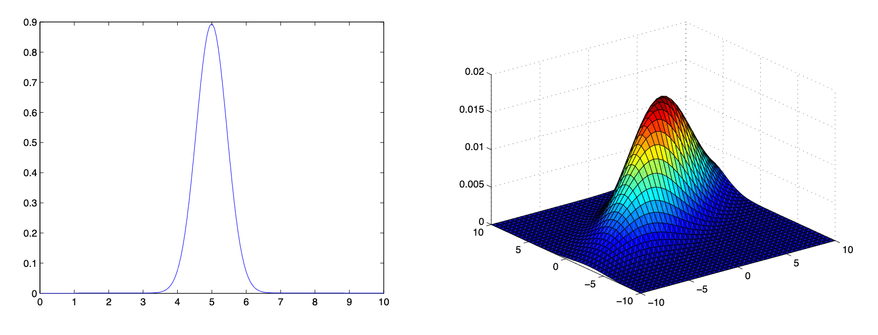
Figure 1: The figure on the left shows a univariate Gaussian density for a single variable X. The figure on the right shows a multivariate Gaussian density over two variables X1 and X2.

The multivariate normal distribution of a $k$-dimensional random vector $\overrightarrow{X}={[X_1,\dots ,X_k]}^{\mathrm{T}}$ can be written in the following notation: $$\overrightarrow{X}\sim \mathcal{N}(\overrightarrow{\mu },\mathrm{\Sigma })$$ or to make it explicitly known that $X$ is $k$-dimensional, $$\overrightarrow{X}\sim {\mathcal{N}}_k(\overrightarrow{\mu },\mathrm{\Sigma })$$ The inverse of the covariance matrix is called the precision matrix, denoted by $Q={\mathrm{\Sigma }}^{-1}$.

The PDF is: $$f_{\overrightarrow{X}}(\overrightarrow{x};\mu ,\mathrm{\Sigma })=\frac{1}{(2\pi {)}^{n/2}|\mathrm{\Sigma }{|}^{1/2}}\exp (-\frac{1}{2}(\overrightarrow{x}-\overrightarrow{\mu }{)}^T{\mathrm{\Sigma }}^{-1}(\overrightarrow{x}-\overrightarrow{\mu }))$$

where $\exp$ denotes the exponential function.

Note:

• $det(\mathrm{\Sigma })$ is the determinant of the covariance matrix.
• ${\mathrm{\Sigma }}^{-1}$ is the inverse of the covariance matrix.

Isocontours

One way to understand a multivariate Gaussian conceptually is to understand the shape of its isocontours. For a function $f:{\mathbf{R}}^2\to \mathbf{R}$, an isocontour is a set of the form $$\{\overrightarrow{x}\in {\mathbf{R}}^2:f(x)=c\}.$$ for some $c\in \mathbf{R}{}^4$.

Shape of isocontours

What do the isocontours of a multivariate Gaussian look like? As before, let's consider the case where $n=2$, and $\mathrm{\Sigma }$ is diagonal, i.e., all the random variables $X_i$ in $\overrightarrow{X}$ are independent (see my post).

Let's take the example of $$\overrightarrow{x}=\left[\begin{array}{l}{x}_1\\ x_2\end{array}\right]\overrightarrow{\mu }=\left[\begin{array}{l}{\mu }_1\\ {\mu }_2\end{array}\right]\mathrm{\Sigma }=\left[\begin{array}{cc}{\sigma }_1^2& 0\\ 0& {\sigma }_2^2\end{array}\right]$$

The PDF is $$f(\overrightarrow{x};\mu ,\mathrm{\Sigma })=\frac{1}{2\pi {\sigma }_1{\sigma }_2}\exp (-\frac{1}{2{\sigma }_1^2}{(x_1-{\mu }_1)}^2-\frac{1}{2{\sigma }_2^2}{(x_2-{\mu }_2)}^2).$$

Now, let's consider the level set consisting of all points where $p(x;\mu ,\mathrm{\Sigma })=c$ for some constant $c\in \mathbf{R}$. In particular, consider the set of all $x_1,x_2\in \mathbf{R}$ such that $$\begin{array}{rl}c& =\frac{1}{2\pi {\sigma }_1{\sigma }_2}\exp (-\frac{1}{2{\sigma }_1^2}{(x_1-{\mu }_1)}^2-\frac{1}{2{\sigma }_2^2}{(x_2-{\mu }_2)}^2)\\ 2\pi c{\sigma }_1{\sigma }_2& =\exp (-\frac{1}{2{\sigma }_1^2}{(x_1-{\mu }_1)}^2-\frac{1}{2{\sigma }_2^2}{(x_2-{\mu }_2)}^2)\\ \log \left(2\pi c{\sigma }_1{\sigma }_2\right)& =-\frac{1}{2{\sigma }_1^2}{(x_1-{\mu }_1)}^2-\frac{1}{2{\sigma }_2^2}{(x_2-{\mu }_2)}^2\\ \log \left(\frac{1}{2\pi c{\sigma }_1{\sigma }_2}\right)& =\frac{1}{2{\sigma }_1^2}{(x_1-{\mu }_1)}^2+\frac{1}{2{\sigma }_2^2}{(x_2-{\mu }_2)}^2\\ 1& =\frac{{(x_1-{\mu }_1)}^2}{2{\sigma }_1^2\log \left(\frac{1}{2\pi c{\sigma }_1{\sigma }_2}\right)}+\frac{{(x_2-{\mu }_2)}^2}{2{\sigma }_2^2\log \left(\frac{1}{2\pi c{\sigma }_1{\sigma }_2}\right)}.\end{array}$$

Defining $$r_1=\sqrt{2{\sigma }_1^2\log \left(\frac{1}{2\pi c{\sigma }_1{\sigma }_2}\right)}{r}_2=\sqrt{2{\sigma }_2^2\log \left(\frac{1}{2\pi c{\sigma }_1{\sigma }_2}\right)},$$ it follows that $$\begin{array}{}\text{(1)}& 1={\left(\frac{x_1-{\mu }_1}{r_1}\right)}^2+{\left(\frac{x_2-{\mu }_2}{r_2}\right)}^2.\end{array}$$

Equation $\text{(1)}$ is the equation of an axis-aligned ellipse, with center $({\mu }_1,{\mu }_2)$, where the $x_1$ axis has length $2r_1$ and the $x_2$ axis has length $2r_2$. ## Length of axes

Figure 2

To get a better understanding of how the shape of the level curves vary as a function of the variances of the multivariate Gaussian distribution, suppose that we are interested in

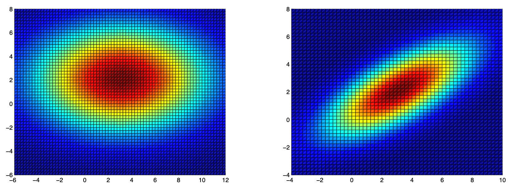
The figure on the left shows a heatmap indicating values of the density function for an axis-aligned multivariate Gaussian with mean $\mu =\left[\begin{array}{l}3\\ 2\end{array}\right]$ and diagonal covariance matrix $\mathrm{\Sigma }=$ $\left[\begin{array}{cr}25& 0\\ 0& 9\end{array}\right]$. Notice that the Gaussian is centered at $(3,2)$, and that the isocontours are all elliptically shaped with major/minor axis lengths in a 5:3 ratio.

The figure on the right shows a heatmap indicating values of the density function for a non axis-aligned multivariate Gaussian with mean $\mu =\left[\begin{array}{l}3\\ 2\end{array}\right]$ and covariance matrix $\mathrm{\Sigma }=\left[\begin{array}{cc}10& 5\\ 5& 5\end{array}\right]$. Here, the ellipses are again centered at $(3,2)$, but now the major and minor axes have been rotated via a linear transformation (because its covariance matrix isn't diagonal), the values of $r_1$ and $r_2$ at which $c$ is equal to a fraction $1/e$ of the peak height of Gaussian density.

First, observe that maximum of Equation (4) occurs where $x_1={\mu }_1$ and $x_2={\mu }_2$. Substituting these values into Equation (4), we see that the peak height of the Gaussian density is $\frac{1}{2\pi {\sigma }_1{\sigma }_2}$. Second, we substitute $c=\frac{1}{e}\left(\frac{1}{2\pi {\sigma }_1{\sigma }_2}\right)$ into the equations for $r_1$ and $r_2$ to obtain $$\begin{array}{rl}& r_1=\sqrt{2{\sigma }_1^2\log \left(\frac{1}{2\pi {\sigma }_1{\sigma }_2\cdot \frac{1}{e}\left(\frac{1}{2\pi {\sigma }_1{\sigma }_2}\right)}\right)}={\sigma }_1\sqrt{2}\\ & r_2=\sqrt{2{\sigma }_2^2\log \left(\frac{1}{2\pi {\sigma }_1{\sigma }_2\cdot \frac{1}{e}\left(\frac{1}{2\pi {\sigma }_1{\sigma }_2}\right)}\right)}={\sigma }_2\sqrt{2}.\end{array}$$

From this, it follows that the axis length needed to reach a fraction 1/e of the peak height of the Gaussian density in the $i$ th dimension grows in proportion to the standard deviation ${\sigma }_i$. Intuitively, this again makes sense: the smaller the variance of some random variable $x_i$, the more "tightly" peaked the Gaussian distribution in that dimension, and hence the smaller the radius $r_i$.

Linear Linear transformation interpretation

Theorem: Let $X\sim \mathcal{N}(\mu ,\mathrm{\Sigma })$ for some $\mu \in {\mathbf{R}}^n$ and $\mathrm{\Sigma }\in {\mathbf{S}}_{++}^n$. Then, there exists a matrix $B\in {\mathbf{R}}^{n\times n}$ such that if we define $Z=B^{-1}(X-\mu )$, then $Z\sim \mathcal{N}(0,I)$.

Proof:

1. As before said, if $Z\sim \mathcal{N}(0,I)$, then it can be thought of as a collection of $n$ independent standard normal random variables (i.e., $Z_i\sim \mathcal{N}(0,1)$ ).
2. Furthermore, if $Z=B^{-1}(X-\mu )$ then $X=BZ+\mu$ follows from simple algebra.
3. Consequently, the theorem states that any random variable $X$ with a multivariate Gaussian distribution can be interpreted as the result of applying a linear transformation $(X=$ $BZ+\mu )$ to some collection of $n$ independent standard normal random variables $(Z)$.

---

1. Probability density function↩︎