DINO: Emerging Properties in Self-Supervised Vision Transformers
Sources:
- Emerging Properties in Self-Supervised Vision Transformers (DINO)
- PyTorch implementation and pretrained models for DINO
Introduction
DINO(shorts for self-distillation with no labels) is a self-supervised pretraining method for visual models like Vision Transformer (ViT)1 and CNN2, while it mainly focus on ViT.
It's trained on ImageNet witout any labels。 It has an amazing video of latent space visualization: https://user-images.githubusercontent.com/46140458/116817761-47885e80-ab68-11eb-9975-d61d5a919e13.mp4
Properties
Features generated by DINO with ViT backbone have following properties
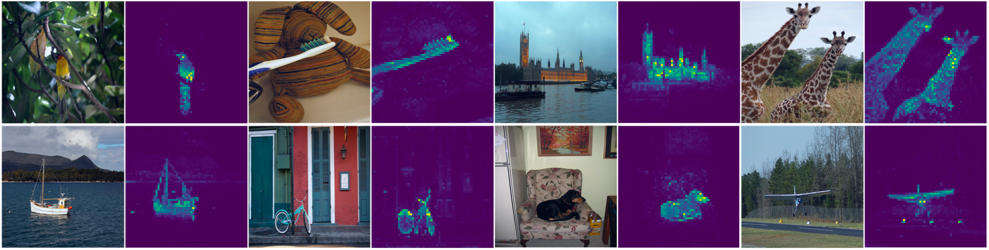
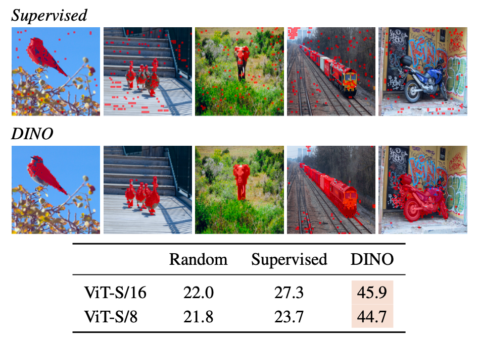
These features explicitly contain the scene layout and, in particular, object boundaries, as shown in Figure 1.
In Figure 1, we look at the self-attention of the
[CLS]token on the heads of the last layer. These maps show that the model automatically learns class-specific features leading to unsupervised object segmentations.These features perform particularly well with a basic nearest neighbors classifier (k-NN) without any finetuning, linear classifier nor data augmentation.
Deno performs well at image segmentation, see Figure 4:
Architecture
Knowledge distillation
DINO is a knowledge distillation method, which typically contains
- A teacher network \(g_{\theta_s}\), parameterized by \(\theta_s\).
- A student network \(g_{\theta_t}\), parameterized by \(\theta_t\).
The goal of knowledge distillation is to to train \(g_{\theta_s}\) to match the output of a given \(g_{\theta_t}\).
However, unlike common distillation methods, in DINO:
- We only train the student network, the teacher network is built by the student network through a method called exponential moving average (EMA).
- Both networks have the same architecture but different parameters. You can see from Figure 2 that a stop-gradient (sg) operator on the teacher is applied to propagate gradients only through the student.
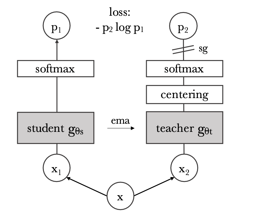
Figure 2 illustrates DINO in the case of one single pair of views \(\left(x_1, x_2\right)\) for simplicity. The model passes two different random transformations of an input image to the student and teacher networks.
We obtain that:
- Each network outputs a \(K\) dimensional feature that is normalized with a temperature softmax over the feature dimension.
- The output of the teacher network is centered with a mean computed over the batch.
- Their similarity is then measured with a cross-entropy loss.
Note: For now you may be confused with terminologies such as EMA, temperature softmax, etc. I'll explain them in the further section.
1 | # DINO PyTorch pseudocode w/o multi-crop. |
Backbone and projection head
A neural network \(g\) is composed of:
- a backbone \(f\) (ViT or ResNet),
- The features used in downstream tasks are the backbone \(f\) output.
- a projection head \(h: g=h \circ f\).
- The projection head consists of a 3-layer multi-layer perceptron (MLP) with hidden dimension 2048 followed by \(\ell_2\) normalization and a weight normalized fully connected layer with \(K\) dimensions.
For ViT
In order to use ViT as our backbone, we have to add an extra learnable token [CLS] to its patch sequence (Recalling that ViT is just another transformer while it use "patches" to form its sequence).
[CLS] is not attached to any label nor supervision.
The role of [CLS] is to aggregate information from the entire sequence and we attach the projection head \(h\) at its output.
Training
Idea of the loss function
Given an input image \(x\), both networks output probability distributions over \(K\) dimensions denoted by \(P_s\) and \(P_t\). The probability \(P\) is obtained by normalizing the output of the network \(g\) with a softmax function. More precisely, for \(P_s\) \[ P_s(x)^{(i)}=\frac{\exp \left(g_{\theta_s}(x)^{(i)} / \tau_s\right)}{\sum_{k=1}^K \exp \left(g_{\theta_s}(x)^{(k)} / \tau_s\right)}, \] with \(\tau_s>0\) a temperature parameter that controls the sharpness of the output distribution.
A similar formula holds for \(P_t\) with temperature \(\tau_t\).
The loss dunction is cross-entropy loss. In Knowledge distillation methods, the teacher network \(g_{\theta_t}\) is given, we train the parameters \(\theta_s\) of the student network: \[ \begin{equation} \label{eq_2} \min _{\theta_s} H\left(P_t(x), P_s(x)\right), \end{equation} \] where \(H(a, b)=-a \log b\).
Loss function (self-supervised)
In the following, we detail how we adapt the problem in \(\eqref{eq_2}\) to self-supervised learning.
First, we do image augmentation with multicrop strategy:
- From a given image \(x\), we generate a set \(V\) of different views. This set contains two global views, \(x_1^g\) and \(x_2^g\) and several local views \(x'\) of smaller resolution.
- Each global view covers a large (for example greater than \(50 \%\) ) area of the original image.
- Each local view covers only small areas (for example less than \(50 \%\) ) of the original image.
- All crops are passed through the student while only the global views are passed through the teacher, therefore encouraging "local-to-global" correspondences.
We minimize the loss: \[ \begin{equation} \label{eq_3} \min _{\theta_s} \sum_{x \in\left\{x_1^g, x_2^g\right\}} \sum_{\substack{x^{\prime} \in V \\ x^{\prime} \neq x}} H\left(P_t(x), P_s\left(x^{\prime}\right)\right) . \end{equation} \]
In experiment, the training method is stochastic gradient descent (SGD).
Note that we only train the student, i.e., in \(\eqref{eq_3}\) we wrote \(\min _{\theta_s}\) instead of \(\min _{\theta_s, \theta_t}\).
How to built the teacher network
One special point of DINO is that its teacher network is not trained. However, it's built from the student weights via a method called exponential moving average (EMA): \[ \theta_t \leftarrow \lambda \theta_t+(1-\lambda) \theta_s \] where \(\lambda\) following a cosine schedule from 0.996 to 1 during training.
Why choose momentum teacher

- Left part:
- Right part: Comparison between different types of teacher network.
To build teacher from, the authors considered 4 methods:
- Using the student network from a previous epoch as a teacher.
- Using the student network from the previous iteration as a teacher.
- Using a copy of student network as a teacher.
- Using EMA to build teacher from the student network.
As shown by right part of Figure 6, which is a comparison between the performance of the momentum teacher and the student during training, the EMA method (momentum method) has the highest performance. So we choose it. (Note that "previous epoch" method also achieves a good performance, which is inetresting.)
Meanwhile, the left part of Figure 6, which is a comparison between different types of teacher network, illustrates that the momentum teacher constantly outperforms the student during the training.
The authors described their method as:
Our method can be interpreted as applying Polyak-Ruppert averaging during the training to constantly build a model ensembling that has superior performances. This model ensembling then guides the training of the student network.
Why DINO can avoid collapse
I don't know... The authors proved this via experiment data, but a theoratical level explanation is absent.
Implementation details
- We pretrain the models on the ImageNet dataset without labels.
- We train with the adamw optimizer and a batch size of 1024, distributed over 16 GPUs when using ViT-S/16.
- The temperature \(\tau_s\) is set to 0.1 while we use a linear warm-up for \(\tau_t\) from 0.04 to 0.07 during the first 30 epochs.
- We follow the data augmentations of BYOL (color jittering, Gaussian blur and solarization) and multi-crop with a bicubic interpolation to adapt the position embeddings to the scales.
- ...
Evaluation protocols
In common, there're 2 protocols for self-supervised learning:
- learning a linear classifier on frozen features
- finetuning the features on downstream tasks
The authors found DINO didn't behave well with either method:
However, both evaluations are sensitive to hyperparameters, and we observe a large variance in accuracy between runs when varying the learning rate for example.
So they adopted a new protocol, where they evaluated the quality of features with a simple weighted \(k-\mathrm{NN}\) classifier:
- Freeze the pretrain model to compute and store the features of the training data of the downstream task.
- The nearest neighbor classifier then matches the feature of an image to the \(k\) nearest stored features that votes for the label.
- In experiment they set \(k=20\)
Differences of DINO and BYOL
- DINO pushes distributions of two embedding closer, i.e., KL divergence loss, instead of pushing two embeddings closer, i.e., MSE or cosine sim.
- Engineer choice.
- DINO seems to not change BYOL very much.