Common Loss Functions
- Cross entropy
- Focal loss
- Hinge loss
- ...
Notations
TO make the context clear, in this article, we make the following regulations:
- The size of the dataset, i.e., the number of the datapoints, is denoted as \(N\).
- The datapoint of index \(i\) is \(x_i \in \mathbb R^{d \times 1}\). The last dimenstion of it is denoted as \(y_i \in \mathbb R^{1 \times 1}\).
- The predicted datapoint by the model is, corresponding to \(x_i\), is \(\hat x_i\). The last dimenstion of it is \(\hat y_i\).
- The predicted value of the \(i^{\text{th}}\) datapoint output by the model is \(p_i\).
- When the task is a classification task, the ground truth value is often a 0/1 label, i.e., \(y_i \in \{0,1\}, \forall i\).
- When the task is a classification task, the number of classes is \(C\). In addition, the ground truth label value and the prediction value of \(c^{\text{th}}\) class of the \(i^{\text{th}}\) datapoint is \(y_{c}, p_{c}\).
Mean Squared Error
Mean squared error (MSE) loss is \[ \mathrm{MSE \ Loss} = \| y_i - \hat y_i \|_2^2=\sqrt{\sum_{i=1}^n\left(y_i- \hat y_i\right)^2} . \]
1 | import torch |
Cross Entropy
For the gradient (or derivation) of Cross Entropy, please refer to ->this article.
--> Youtube: Cross Entropy
Cross-entropy loss (often abbreviated as CE), or log loss, measures the performance of a classification model whose output is a probability value between 0 and 1 (usually produced by a softmax function).
The cross entropy loss \(L\) of a sample is \[ L = -\sum_{i=1}^C y_{i} \log \left(\hat y_{i}\right) . \]
where \(\hat{y}_i\) is the predicted probability for class \(i\), usually obtained by applying the softmax function to the logits For classification tasks where there is only one true class for a sample, i.e., \(y_c \in \{0,0, \cdots, 1, 0, \cdots \}\), suppose the index of the true class of the input data point is \(t\), we obtain \[ L=- (0 + \cdots + 0+1 \cdot \log (\hat y_t) + 0 + \cdots+0) = - \log (\hat y_t) \]
1 | import torch |
Example
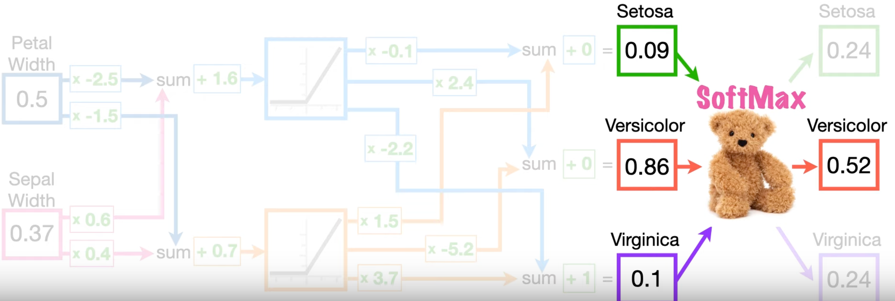
For example, consider following neural network, there're three data points "Setosa", "Virginica" and "Versicolor", each is a 2-D vector. The number of classes is \(N = 3\) since softmax outputs 3 values.
| Petal | Sepal | Species | \(p\) | Cross Entropy |
|---|---|---|---|---|
| 0.04 | 0.42 | Setosa | 0.57 | \(1 . ({-\log (p)}) + 0 + 0 =0.56\) |
| 1 | 0.54 | Virginica | 0.58 | $ 0 + 1. {-(p)} + 0 =0.54$ |
| 0.50 | 0.37 | Versicolor | 0.52 | \(0 + 0 + -\log (p)=0.65\) |
Take Sepal for Versicolor, when input is Versicolor (\([0.50, 0.37]\)), the true label value of Versicolor is \(1\) and that of others is all \(0\). \[ \begin{aligned} y_{\text{Setosa}} = 0, \\ y_{\text{Virginica}} = 0, \\ y_{\text{Versicolor}} = 1, \end{aligned} \] The output of softmax corresponding to Versicolor is \(p_{\text{Versicolor}} = 0.52\).
Therefore, the cross entropy of this training is \[ 1 . ({-\log (p)}) + 0 + 0 =0.56 . \]
Property
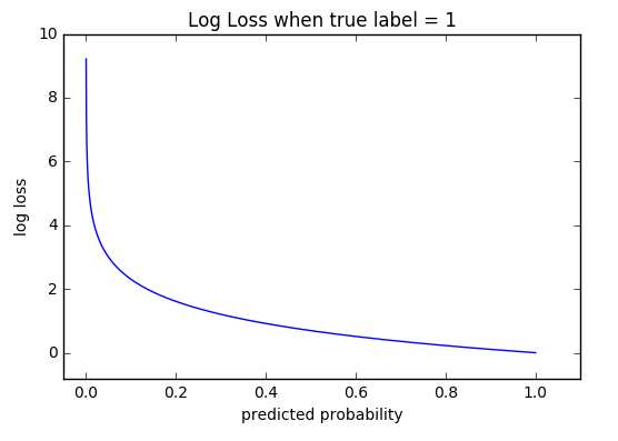
The graph above shows the range of possible loss values given a true observation (isDog = 1). As the predicted probability approaches 1, log loss slowly decreases. As the predicted probability decreases, however, the log loss increases rapidly.
Log loss heavily penalizes those predictions that are confident and wrong.
Problems
The main problem of cross entropy is that, even when the prediction is correct, i.e., y_predicted == y_true, the cross entropy isn't symmetric.
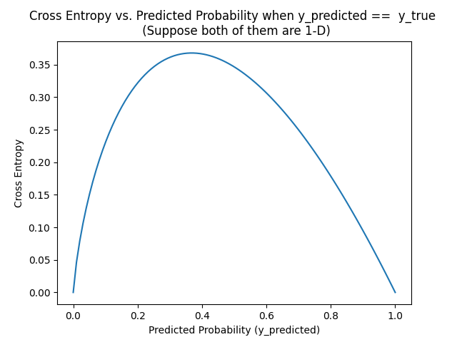
From this figure, if y_predicted == y_true == 0.2, their CE is 0.3218.... If y_predicted == y_true == 0.8, their CE is 0.178514. They're not equal!
Focal Loss
--> Focal Loss for Dense Object Detection
A Focal Loss function addresses (extreme) class imbalance during training in tasks like object detection. Focal loss applies a modulating term to the cross entropy loss in order to focus learning on hard misclassified examples.
Formally, the Focal Loss adds a factor \(\left(1-\hat y_t\right)^\gamma\) to the standard cross entropy criterion. \[ \mathrm{FL}\left(\hat y_t\right)=-\left(1- \hat y_t\right)^\gamma \log \left( \hat y_t\right) \]
Property
(In the below figure, the notation \(\hat y\) is replaced by \(p\))
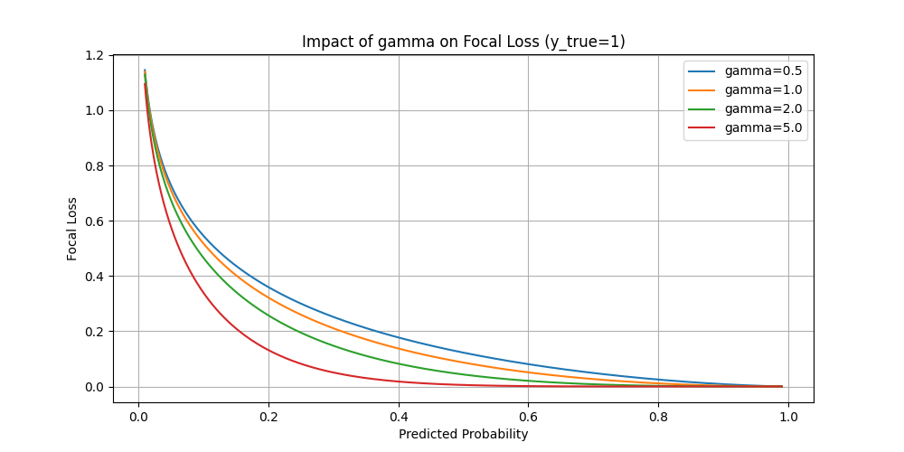
- Setting \(\gamma>0\) reduces the relative loss for well-classified examples \(\left(\hat y_t>.5\right)\), putting more focus on hard, misclassified examples. Here there is tunable focusing parameter \(\gamma \geq 0\).
- One typical use case is in object detection tasks. An image may contain 5 onjects whereas the the number of bounding boxes can be millions. Thus there're enormous negative datapoints. The model can easily learn to judge all data points to be false to achieve a high traing performance.
1 | import torch |
Dice Loss
--> Source
Dice Loss was originally designed for binary classification problems, particularly in the context of binary segmentation where you're often distinguishing between the foreground and the background.
Dice Coefficient
It's derived from Dice Coefficient, which is a statistic used to gauge the similarity of two samples.
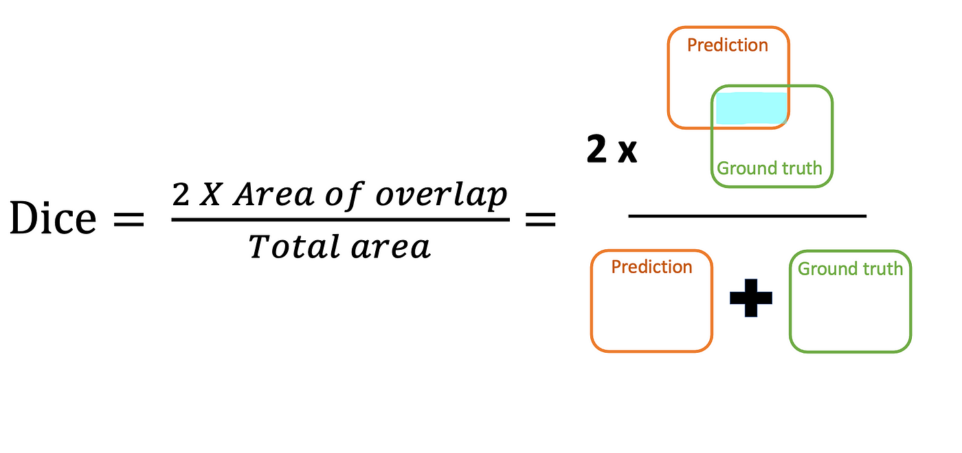 For the \(i^{\text{th}}\) datapoint, the Dice Coefficient is \[
\mathrm{Dice}=\frac{2 \times \sum_i \left(\hat y_i \times y_i\right)}{\sum_i \hat y_i+\sum_i y_i} .
\]
For the \(i^{\text{th}}\) datapoint, the Dice Coefficient is \[
\mathrm{Dice}=\frac{2 \times \sum_i \left(\hat y_i \times y_i\right)}{\sum_i \hat y_i+\sum_i y_i} .
\]
1 | def dice_coef(groundtruth_mask, pred_mask): |
Dice Loss
The Dice Loss is \[ \mathrm{DL} = 1 - \mathrm{Dice} . \]
1 | def dice_loss(groundtruth_mask, pred_mask): |
IoU
--> Source
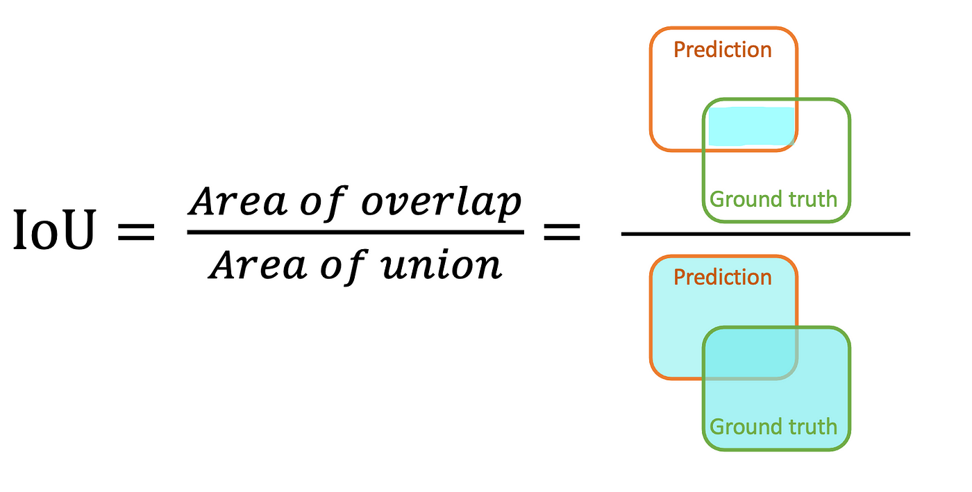
Jaccard index, also known as Intersection over Union (IoU), is the area of the intersection over union of the predicted segmentation and the ground truth \[ \mathrm{I o U}=\frac{T P}{T P+F P+F N} \]
1 | def iou(groundtruth_mask, pred_mask): |