Bellman Equation

Posted on 2024-01-03 Edited on 2024-09-17 In Computer Science Views:

Sources:

Shiyu Zhao. Chapter 2: State Values and Bellman Equation. Mathematical Foundations of Reinforcement Learning.
--> Youtube: Bellman Equation: Derivation

Problem Formula

Given a policy, finding out the corresponding state values is called policy evaluation. This is through solving an equation called the Bellman equation.

State Value

The expectation (or expected value, mean) of $G_t$ is defined as the state-value function or simply state value: \[ \begin{equation} \label{eq_def_of_state_value} v_\pi(s)=\mathbb{E}\left[G_t \mid S_t=s\right] \end{equation} \]

Remarks:

It is a function of $s$. It is a conditional expectation with the condition that the state starts from $s$.
Since $G_t$ is based on some policy $\pi$, its expectation $v_\pi(s)$ is also based on some policy $\pi$, i.e., for a different policy, the state value may be different.
It represents the "value" of a state. If the state value is greater, then the policy is better because greater cumulative rewards can be obtained.

Derivation of the Bellman equation

Recalling the definition of the state value $\eqref{eq_def_of_state_value}$, we substitute \[ G(t) = R_{t+1}+\gamma G_{t+1} \] into it¹:

\[ \begin{aligned} \label{eq_derivation_of_state_value_function} v_\pi(s) & =\mathbb{E}[G_t \mid S_t=s] \\ & =\mathbb{E}[R_{t+1}+\gamma G_{t+1} \mid S_t=s] \\ & =\color{teal}{\mathbb{E} [R_{t+1} \mid S_t=s]}+ \gamma \color{salmon}{\mathbb{E}[G_{t+1} \mid S_t=s]} \end{aligned} \]

The two terms in the last line of are analyzed below.

First term: the mean of immediate rewards

First, calculate the first term $\mathbb{E}\left[R_{t+1} \mid S_t=s\right]$ : \[ \begin{aligned} \color{teal}{\mathbb{E}\left[R_{t+1} \mid S_t=s\right]} & =\sum_{a \in \mathcal A(s)} \pi(a \mid s) \mathbb{E}\left[R_{t+1} \mid S_t=s, A_t=a\right] \\ & = \color{teal}{\sum_{a \in \mathcal A(s)} \pi(a \mid s) \sum_r p(r \mid s, a) r} . \end{aligned} \]

This is the mean of immediate rewards.

Explanation

Given events $R_{t+1} = r, S_t = s, A_t = a$, the deduction is quite simple.

From the law of total expectation: given discrete random variables $X$ and $Y$, then \[ \mathbb{E}(X)=\mathbb{E}(\mathbb{E}(X \mid Y)) \] If $Y$ is finite, we have \[ \mathbb{E}(X)=\sum_{y_i \in \mathcal{Y}} \mathbb{E}\left(X \mid Y=y_i\right) p\left(Y=y_i\right) \] where $\mathcal Y$ is the alphabet of $Y$.

Thus we obtain: \[ \mathbb{E}\left[R_{t+1} \mid S_t=s\right] =\sum_{a \in \mathcal A(s)} \pi(a \mid s) \mathbb{E}\left[R_{t+1} \mid S_t=s, A_t=a\right] \] where $A_t$ is finite.
From the definition of expectation, $\mathbb{E}\left[R_{t+1} \mid S_t=s, A_t=a\right] = p(r \mid s, a) r$, leading to \[ \sum_{a \in \mathcal A(s)} \pi(a \mid s) \mathbb{E}\left[R_{t+1} \mid S_t=s, A_t=a\right] = \sum_{a \in \mathcal A(s)} \pi(a \mid s) \sum_r p(r \mid s, a) r \] Q.E.D.

A more verbose version of deduction is:

First, consider the definition of expectation: \[ \begin{equation} \label{eq_def_of_expectation} \mathbb{E}\left[R_{t+1} \mid S_t=s\right] \triangleq \sum_r p(r | s) r. \end{equation} \] Look at use the formula for marginal probability, \[ p(r | s) = \sum_{a \in \mathcal A(s)} p(r, a| s). \] Due to the chain rule of probability, we obtain \[ p(r, a| s) = p(r | a, s). p(a|s) \] And in RL context, $p(s|s)$ is often written as $\pi(a|s)$.

Therefore, \[ p(r | s) = \sum_{a \in \mathcal A(s)} \pi(a|s) . p(r | a, s) \]

Replace $p(r | s)$ in $\eqref{eq_def_of_expectation}$ with $\sum_{a \in \mathcal A(s)} \pi(a|s) . p(r | a, s)$, we get \[ \begin{aligned} \mathbb{E}\left[R_{t+1} \mid S_t\right] &= \sum_r \sum_{a \in \mathcal A(s)} \pi(a \mid s) p(r \mid s, a) r \\ &= \sum_{a \in \mathcal A(s)} \pi(a \mid s) \sum_r p(r \mid s, a) r \\ & \triangleq \sum_{a \in \mathcal A(s)} \pi(a \mid s) \mathbb{E}\left[R_{t+1} \mid S_t=s, A_t=a\right] \\ \end{aligned} \]

Q.E.D.

Second term: the (discounted) mean of future rewards

First, we calculate the mean of future rewards \[ \begin{aligned} \mathbb{E}\left[G_{t+1} \mid S_t=s\right] & =\sum_{s^{\prime}} \mathbb{E}\left[G_{t+1} \mid S_t=s, S_{t+1}=s^{\prime}\right] p\left(s^{\prime} \mid s\right) \\ & =\sum_{s^{\prime}} \mathbb{E}\left[G_{t+1} \mid S_{t+1}=s^{\prime}\right] p\left(s^{\prime} \mid s\right) \\ & =\sum_{s^{\prime}} v_\pi\left(s^{\prime}\right) p\left(s^{\prime} \mid s\right) \\ & =\sum_{s^{\prime}} v_\pi\left(s^{\prime}\right) \sum_a p\left(s^{\prime} \mid s, a\right) \pi(a \mid s) \end{aligned} \]

Then we multiply it with a dicount factor $\gamma$. For simplicity, we say the second term $\gamma \mathbb{E}[G_{t+1} \mid S_t$ is "the mean of future rewards" also it's discounted.

Explanation

The transotion of the first line comes from the law of total expectation as well.

The transotion of the second line comes from the Markov property. Recall that reward $r_t$ is defined to only rely on $s_t$ and $a_t$: \[ p\left(r_{t+1} \mid s_t, a_t, s_{t-1}, a_{t-1}, \ldots, s_0, a_0\right)=p\left(r_{t+1} \mid s_t, a_t\right) . \] We obtain that $$ \[\begin{aligned} \mathbb E[R_{t+1} \mid s_t, a_t, s_{t-1}, a_{t-1}, \ldots, s_0, a_0] & \triangleq \sum_{r_{t+1} \in \mathcal {R_{t+1}}} p(r_{t+1} \mid s_t, a_t, s_{t-1}, a_{t-1}, \ldots, s_0, a_0) \cdot r_{t+1} \\ & = \sum_{r_{t+1} \in \mathcal {R_{t+1}}} p(r_{t+1} \mid s_t, a_t) \cdot r_{t+1} \\ & \triangleq \mathbb E[R_{t+1} \mid s_t, a_t] . \end{aligned}\] \[ Since \] G_t = R_{t+1}+R_{t+2}+^2 R_{t+3}+, \[ we have \] \[\begin{aligned} \mathbb{E}[G_{t+1} \mid S_t=s, S_{t+1}=s^{\prime}] & = \mathbb{E}[R_{t+1}+\gamma R_{t+2}+\gamma^2 R_{t+3}+\ldots \mid S_t=s, S_{t+1}=s^{\prime}] \\ & = \mathbb{E}[R_{t+1}+\gamma R_{t+2}+\gamma^2 R_{t+3}+\ldots \mid S_{t+1}=s^{\prime}] \end{aligned}\]

Bellman equation

Therefore, we have the Bellman equation, $$ \[\begin{aligned} v_\pi(s) & =\mathbb{E}\left[R_{t+1} \mid S_t=s\right]+\gamma \mathbb{E}\left[G_{t+1} \mid S_t=s\right], \\ & = \underbrace{\color{teal}\sum_a \pi(a \mid s) \sum_r p(r \mid s, a) r}_{\text {mean of immediate rewards }} + \underbrace{\gamma \color{salmon} {\sum_{s^{\prime}} \pi(a \mid s) \sum_a p\left(s^{\prime} \mid s, a\right) v_\pi\left(s^{\prime}\right)},}_{\text {(discounted) mean of future rewards }} \\ & =\sum_a \pi(a \mid s)\left[\sum_r p(r \mid s, a) r+\gamma \sum_{s^{\prime}} p\left(s^{\prime} \mid s, a\right) v_\pi\left(s^{\prime}\right)\right], \quad \forall s \in \mathcal{S} . \end{aligned}\]

It consists of two terms:
1. First term: the mean of immediate rewards
2. Second term: the (discounted )mean of future rewards
The Bellman equation is a set of linear equations that describe the relationships between the values of all the states.
The above elementwise form is valid for every state $s \in \mathcal{S}$. That means there are $|\mathcal{S}|$ equations like this!

Examples

Refer to the grid world example for the notations.

For deterministic policy

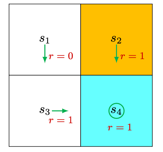
Figure 2.4: An example for demonstrating the Bellman equation. The policy in this example is deterministic.

Consider the first example shown in Figure 2.4, where the policy is deterministic. We next write out the Bellman equation and then solve the state values from it.

First, consider state $s_1$. Under the policy, the probabilities of taking the actions are \[ \pi\left(a=a_3 \mid s_1\right)=1 \quad \text{and} \quad \pi\left(a \neq a_3 \mid s_1\right)=0. \] The state transition probabilities are \[ p\left(s^{\prime}=s_3 \mid s_1, a_3\right)=1 \quad \text{and} \quad p\left(s^{\prime} \neq s_3 \mid s_1, a_3\right)=0 . \]

The reward probabilities are \[ p\left(r=0 \mid s_1, a_3\right)=1 \quad \text{and} \quad p\left(r \neq 0 \mid s_1, a_3\right)=0 . \]

Substituting these values into the Bellman equation mentioned before \[ v_\pi (s) = \sum_a \pi(a \mid s)\left[\sum_r p(r \mid s, a) r+\gamma \sum_{s^{\prime}} p\left(s^{\prime} \mid s, a\right) v_\pi\left(s^{\prime}\right)\right], \quad \forall s \in \mathcal{S} \] gives \[ v_\pi\left(s_1\right)=0+\gamma v_\pi\left(s_3\right) \]

Similarly, it can be obtained that \[ \begin{aligned} & v_\pi\left(s_2\right)=1+\gamma v_\pi\left(s_4\right), \\ & v_\pi\left(s_3\right)=1+\gamma v_\pi\left(s_4\right), \\ & v_\pi\left(s_4\right)=1+\gamma v_\pi\left(s_4\right) . \end{aligned} \]

We can solve the state values from these equations. Since the equations are simple, we can manually solve them. More complicated equations can be solved by the algorithms presented later. Here, the state values can be solved as \[ \begin{aligned} & v_\pi\left(s_4\right)=\frac{1}{1-\gamma}, \\ & v_\pi\left(s_3\right)=\frac{1}{1-\gamma}, \\ & v_\pi\left(s_2\right)=\frac{1}{1-\gamma}, \\ & v_\pi\left(s_1\right)=\frac{\gamma}{1-\gamma} . \end{aligned} \] Furthermore, if we set $\gamma=0.9$, then \[ \begin{aligned} & v_\pi\left(s_4\right)=\frac{1}{1-0.9}=10, \\ & v_\pi\left(s_3\right)=\frac{1}{1-0.9}=10, \\ & v_\pi\left(s_2\right)=\frac{1}{1-0.9}=10, \\ & v_\pi\left(s_1\right)=\frac{0.9}{1-0.9}=9 . \end{aligned} \]

For stochastic policy

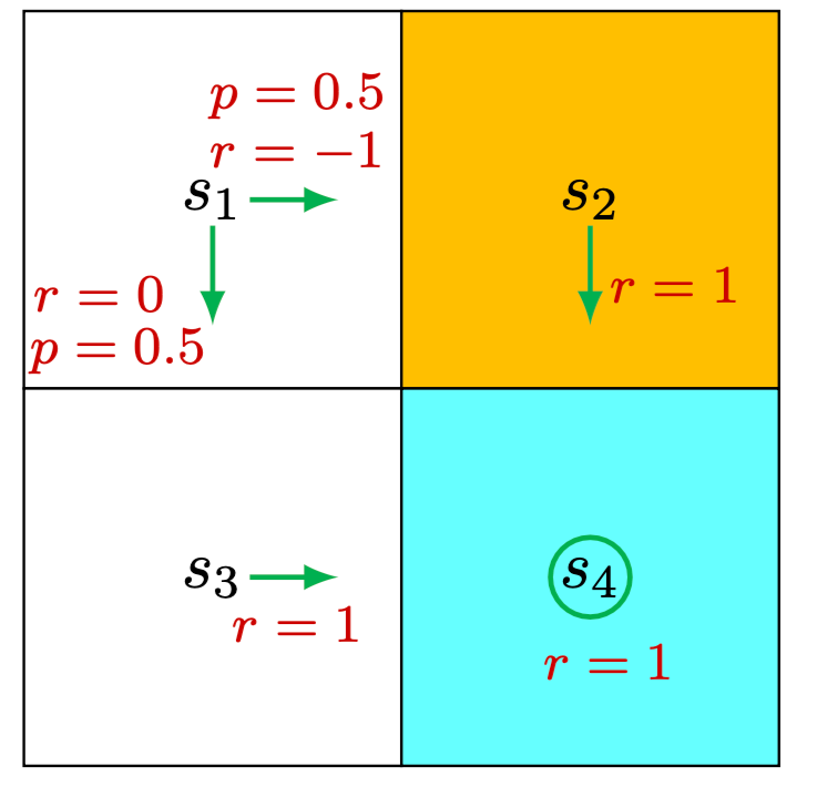
Figure 2.5: An example for demonstrating the Bellman equation. The policy in this example is stochastic.

Consider the second example shown in Figure 2.5, where the policy is stochastic. We next write out the Bellman equation and then solve the state values from it.

At state $s_1$, the probabilities of going right and down equal 0.5 . Mathematically, we have $\pi\left(a=a_2 \mid s_1\right)=0.5$ and $\pi\left(a=a_3 \mid s_1\right)=0.5$. The state transition probability is deterministic since $p\left(s^{\prime}=s_3 \mid s_1, a_3\right)=1$ and $p\left(s^{\prime}=s_2 \mid s_1, a_2\right)=1$. The reward probability is also deterministic since $p\left(r=0 \mid s_1, a_3\right)=1$ and $p\left(r=-1 \mid s_1, a_2\right)=1$. Substituting these values into (2.7) gives \[ v_\pi\left(s_1\right)=0.5\left[0+\gamma v_\pi\left(s_3\right)\right]+0.5\left[-1+\gamma v_\pi\left(s_2\right)\right] \]

The state values can be solved from the above equations. Since the equations are

simple, we can solve the state values manually and obtain \[ \begin{aligned} v_\pi\left(s_4\right) & =\frac{1}{1-\gamma}, \\ v_\pi\left(s_3\right) & =\frac{1}{1-\gamma}, \\ v_\pi\left(s_2\right) & =\frac{1}{1-\gamma}, \\ v_\pi\left(s_1\right) & =0.5\left[0+\gamma v_\pi\left(s_3\right)\right]+0.5\left[-1+\gamma v_\pi\left(s_2\right)\right], \\ & =-0.5+\frac{\gamma}{1-\gamma} . \end{aligned} \]

Furthermore, if we set $\gamma=0.9$, then \[ \begin{aligned} & v_\pi\left(s_4\right)=10, \\ & v_\pi\left(s_3\right)=10, \\ & v_\pi\left(s_2\right)=10, \\ & v_\pi\left(s_1\right)=-0.5+9=8.5 . \end{aligned} \]

In this article we only deal with discounted return witout the loss of generality since we can simply trate undiscounted return as discounted-return's special case when $\gamma = 1$.↩︎