Basic Concepts in Reinforcement Learning
Sources:
- Shiyu Zhao. Chapter 1: Basic Concepts. Mathematical Foundations of Reinforcement Learning.
- OpenAI Spinning Up
Notation
Here I list the notations I use in my Reinforcement Learning (RL) posts. We follow the conventions in probability theory such that
- Samples are denoted as lower-case italicized Roman letters, such as \(s, a, r\).
- Sample Spaces are denoted by upper-case calligraphic fonts, such as \(\mathcal S, \mathcal A, \mathcal R\).
- Random variables are denoted by upper-case italicized Roman letters, such as \(S, A, R\).
| Symbol | Meaning |
|---|---|
| \(s\) | The state of an environment. |
| \(a\) | The action to take by the agent. |
| \(r\) | The reward an agent obtains after executing an action at a state. The reward must be a scalar. |
| \(o\) | The observation \(o\) if an environment. It is a partial description of a state, which may omit information. |
| \(S\) | The random variable reprsenting the state of an environment. |
| \(O\) | The random variable reprsenting the observation of an environment. |
| \(A\) | The random variable reprsenting the action to take by the agent. |
| \(R\) | The random variable reprsenting the reward an agent obtains after executing an action at a state. The reward must be a scalar. Note that we have \(S_t \xrightarrow{A_t} R_{t+1}\), i.e., for state and action at time index \(t\), the reward is at the next time index \(t+1\), not \(t\). |
| \(s_t, o_t, a_t, r_t\) | The state, observation, action, reward at time index \(t\) are denoted as \(s_t, o_t, a_t, r_t\) separately. |
| \(S_t, O_t, A_t, R_t\) | The random variables representing the state, observation, action, reward at time index \(t\) are denoted as \(S_t, O_t, A_t, R_t\) separately. |
| \(r(s, a)\) | The reward is a function of the state \(s\) and action \(a\). Hence, it is also denoted as \(r(s, a)\). |
| \(R(s, a)\) | For the same reson, the reward random vaiable is also denoted as \(R(s, a)\). |
| \(\mathcal{S}\) | The set of all states, called the state space. We have \(s \in {\mathcal S}\). |
| \(\mathcal{A}\) | The set of all actions, called the action space. We have \(a \in {\mathcal A}\). |
| \(\mathcal{R}\) | The set of all rewards, called the reward space. We have \(r \in {\mathcal R}\). |
| \(\mathcal{A}(s)\) | It's common that an action space is associated with the state \(s \in \mathcal{S}\). In this case, the action space is denoted as \(\mathcal{A}(s)\). |
| \(\mathcal{R}(s, a)\) | It's common that a reward space is associated with the state and action (called the each state-action pair \((s, a)\)). In this case, the reward space is denoted as \(\mathcal{R}(s, a)\). |
| \(\mu\) | The policy of an agent. By convention, we use \(\mu\) to denote a deterministic policy. The deterministic policy for a state \(s\) is \(\mu(s)\). |
| \(\pi\) | The policy of an agent. By convention, we use \(\pi\) to denote a stochastic policy. The stochastic policy for a state \(s\) is \(\pi(s)\). |
| \(\tau\) | The trajectory, which is a state-action chain \(\tau = (s_1, a_1, s_2, a_2, ...)\). |
| \(g\) | The return (or cumulative rewards) of a trajetory. We often consider a discounted return with a discount rate \(\gamma \in (0,1)\). We have \(g_t =r_{t+1}+\gamma r_{t+2}+\ldots\). Note that \(r_{t+1}\) is the reward of arriving state \(s_{t+1}\) (or leaving \(s_t\)). |
| \(G\) | The random variable reprsenting the return (or cumulative rewards) of a trajetory. |
| \(g_t\) | Suppose the trajectory starts from time index \(t\), its return is denoted as \(g_t\). |
| \(G_t\) | The random variable reprsenting the return of a trajectory starting from time index \(t\). |
| \(G(\tau)\) or \(R(\tau)\) | The return is a function of the trajectory \(\tau\). Hence, it is also denoted as \(G(s, a)\) (or \(R(\tau)\) since return is just discunted cumulative rewards). |
| \(v_\pi(s)\) | The function \(v_\pi(s)\) is called the state value function. It is the expectation of \(g\) starting from state \(s\). For a specific state \(s\), the value of \(v_\pi(s)\) is called the state value of \(s\). |
A grid world example
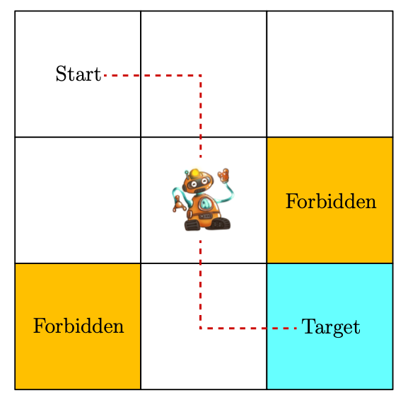
Another important example we use in our posts is the grid world example, shown in Figure 1.2, where a robot moves in a grid world. The robot, called agent, can move across adjacent cells in the grid. At each time step, it can only occupy a single cell.
The white cells are accessible for entry, and the orange cells are forbidden. There is a target cell that the robot would like to reach. We will use such grid world examples throughout this RL serie since they are intuitive for illustrating new concepts and algorithms.
State and action
The concept state describes the agent's status with respect to the environment. The set of all the states is called the state space, denoted as \(\mathcal{S}\).
For each state, the agent can take (may be different) actions. The set of all actions is called the action space, denoted as \(\mathcal{A}\) (or more precisely, \(\mathcal{A}(s)\) when at state \(s\)).
In the grid world example, the state corresponds to the agent's location. Since there are nine cells, there are nine states as well, thus \(\mathcal{S}=\left\{s_1, \ldots, s_9\right\}\).
For each state, the agent can take five possible actions: moving upward, moving rightward, moving downward, moving leftward, and remaining unchanged. These five actions are denoted as \(a_1, a_2, \ldots, a_5\), respectively, thus \(\mathcal{A}=\left\{a_1, \ldots, a_5\right\}\).
Considering that taking \(a_1\) or \(a_4\) at state \(s_1\) would lead to a collision with the boundary, we can set the action space for state \(s_1\) as \(\mathcal{A}\left(s_1\right)=\left\{a_2, a_3, a_5\right\}\).
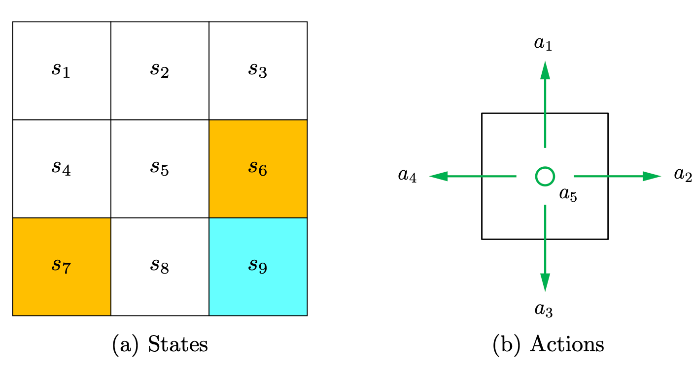
In this RL serie, we consider the most general case: \(\mathcal{A}\left(s_i\right)=\mathcal{A}=\left\{a_1, \ldots, a_5\right\}\) for all \(i\).
States and Observations
You may see the terminology "observation". It's similar to "states". Wha's the difference?
A state \(s\) is a complete description of the state of the world. There is no information about the world which is hidden from the state.
An observation \(o\) is a partial description of a state, which may omit information.
The environment is fully observed when the agent is able to observe the complete state of the environment.
The environment is partially observed when the agent can only see a partial observation.
Reinforcement learning notation sometimes puts the symbol for state,  , in places where it would be technically more appropriate to write the symbol for observation, \(o\).
Specifically, this happens when talking about how the agent decides an action: we often signal in notation that the action is conditioned on the state, when in practice, the action is conditioned on the observation because the agent does not have access to the state.
In our guide, we’ll follow standard conventions for notation, but it should be clear from context which is meant. If something is unclear, though, please raise an issue! Our goal is to teach, not to confuse.
State transition
When taking an action, the agent may move from one state to another. Such a process is called state transition. For example, if the agent is at state \(s_1\) and selects action \(a_2\) (that is, moving rightward), then the agent moves to state \(s_2\). Such a process can be expressed as \[ s_1 \stackrel{a_2}{\rightarrow} s_2 \]
We next examine two important examples.
- What is the next state when the agent attempts to go beyond the boundary, for example, taking action \(a_1\) at state \(s_1\) ? The answer is that the agent will be bounced back because it is impossible for the agent to exit the state space. Hence, we have \(s_1 \stackrel{a_1}{\rightarrow} s_1\).
- What is the next state when the agent attempts to enter a forbidden cell, for example, taking action \(a_2\) at state \(s_5\) ? Two different scenarios may be encountered.
- In the first scenario, although \(s_6\) is forbidden, it is still accessible. In this case, the next state is \(s_6\); hence, the state transition process is \(s_5 \stackrel{a_2}{\longrightarrow} s_6\).
- In the second scenario, \(s_6\) is not accessible because, for example, it is surrounded by walls. In this case, the agent is bounced back to \(s_5\) if it attempts to move rightward; hence, the state transition process is \(s_5 \stackrel{a_2}{\rightarrow} s_5\).
- Which scenario should we consider? The answer depends on the physical environment. In this serie, we consider the first scenario where the forbidden cells are accessible, although stepping into them may get punished. This scenario is more general and interesting. Moreover, since we are considering a simulation task, we can define the state transition process however we prefer. In real-world applications, the state transition process is determined by real-world dynamics.
Policy
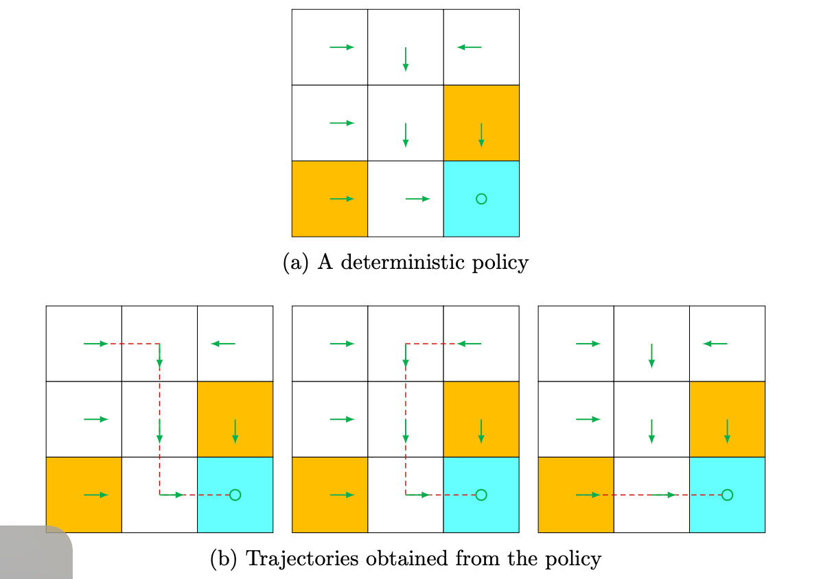
A policy tells the agent which actions to take at every state. Intuitively, policies can be depicted as arrows (see Figure 1.4(a)). Following a policy, the agent can generate a trajectory starting from an initial state (see Figure 1.4(b)).
A policy can be deterministic or stochastic.
Deterministic policy
A deterministic policy is usually denoted by \(\mu\) : \[ a_t=\mu\left(s_t\right) . \]
Stochastic policy
A stochastic policy is usually denoted by \(\pi\) : \[ a_t \sim \pi\left(\cdot \mid s_t\right) . \] In this case, at state \(s\), the probability of choosing action \(a\) is \(\pi(a \mid s)\). It holds that \(\sum_{a \in \mathcal{A}(s)} \pi(a \mid s)=1\) for any \(s \in \mathcal{S}\).
It is preferrable to use \(\pi\) because stochastic policies are more common.
Meanwhile, the policies are often parameterized, the parameters are commonly denoted as \(\theta\) or \(\phi\) and are written as a subscript on the policy symbol:
\[ \begin{aligned} a_t & = \mu_{\theta}(s_t) \\ a_t & \sim \pi_{\theta}(\cdot | s_t). \end{aligned} \]
Reward
After executing an action at a state, the agent obtains a reward, denoted as \(r\), as feedback from the environment.
The reward is a function of the state \(s\) and action \(a\). Hence, it is also denoted as \(r(s, a)\). Its value can be a positive or negative real number or zero.
In the grid world example, the rewards are designed as follows:
- If the agent attempts to exit the boundary, let \(r_{\text {boundary }}=-1\).
- If the agent attempts to enter a forbidden cell, let \(r_{\text {forbidden }}=-1\).
- If the agent reaches the target state, let \(r_{\text {target }}=+1\).
- Otherwise, the agent obtains a reward of \(r_{\text {other }}=0\).
Trajectory
A trajectory \(\tau\) is a state-action chain \(\tau = (s_1, a_1, s_2, a_2, ...)\).
Note that the trajectory is based on some policy \(\pi\), since at every state, the agent selects action based on its policy.
Return
We also define the return of a trajectory as the sum of all the rewards collected along the trajectory. It's undiscounted. However, it's more common to consider discounted return with a discount rate \(\gamma \in (0,1)\):
Consider a trajectory: \[ S_t \xrightarrow{A_t} R_{t+1}, S_{t+1} \stackrel{A_{t+1}}{\longrightarrow} R_{t+2}, S_{t+2} \stackrel{A_{t+2}}{\longrightarrow} R_{t+3}, \ldots \]
The (often discounted) return is denoted as \(G_t\): \[ \begin{aligned} G_t & =R_{t+1}+\gamma R_{t+2}+\gamma^2 R_{t+3}+\ldots \\ & =R_{t+1}+\gamma\left(R_{t+2}+\gamma R_{t+3}+\ldots\right) \\ & =R_{t+1}+\gamma G_{t+1} . \end{aligned} \]
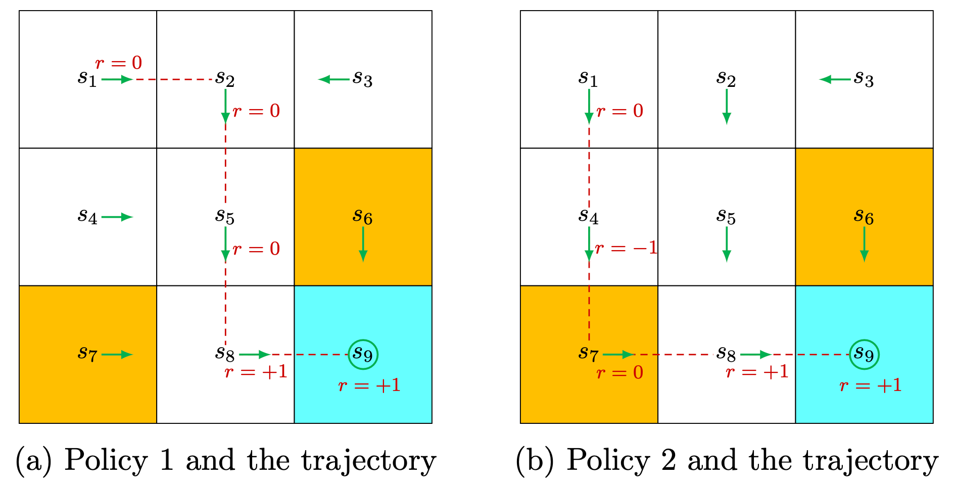
Returns are also called total rewards or cumulative rewards. \[ s_1 \underset{r=0}{\stackrel{a_2}{\longrightarrow}} s_2 \underset{r=0}{\stackrel{a_3}{\longrightarrow}} s_5 \underset{r=0}{\stackrel{a_3}{\longrightarrow}} s_8 \underset{r=1}{\stackrel{a_2}{\longrightarrow}} s_9 . \]
The (undiscounted) return of this trajectory is \[ \text { return }=0+0+0+1=1 . \] The discounted return with a discount rate \(\gamma \in (0,1)\) of this trajectory is \[ \text { return }= 0+ \gamma 0+ \gamma^2 0+ \gamma^3 1 = \gamma^3 . \]
NOTE: The return is based on the trajectory, and the trajectory is based on a policy. Thus, the return is based one a policy as well.
Episode
When interacting with the environment by following a policy, the agent may stop at some terminal states. In this case, the resulting trajectory is finite, and is called an episode (or a trial, rollout).
However, some tasks may have no terminal states. In this case, the resulting trajectory is infinite.
Tasks with episodes are called episodic tasks. Tasks are called continuing tasks.
In fact, we can treat episodic and continuing tasks in a unified mathematical manner by converting episodic tasks to continuing ones. We have two options:
- First, if we treat the terminal state as a special state, we can specifically design its action space or state transition so that the agent stays in this state forever. Such states are called absorbing states, meaning that the agent never leaves a state once reached.
- Second, if we treat the terminal state as a normal state, we can simply set its action space to the same as the other states, and the agent may leave the state and come back again. Since a positive reward of \(r=1\) can be obtained every time \(s_9\) is reached, the agent will eventually learn to stay at \(s_9\) forever (self-circle) to collect more rewards.
In this RL serie, we consider the second scenario where the target state is treated as a normal state whose action space is \(\mathcal{A}\left(s_9\right)=\left\{a_1, \ldots, a_5\right\}\).
Markov decision process
This section presents the basic RL concepts in a more formal way under the framework of Markov decision processes (MDPs).
An MDP is a general framework for describing stochastic dynamical systems. The key ingredients of an MDP are listed below.
Sets:
- State space: the set of all states, denoted as \(\mathcal{S}\).
- Action space: a set of actions, denoted as \(\mathcal{A}(s)\), associated with each state \(s \in \mathcal{S}\).
- Reward set: a set of rewards, denoted as \(\mathcal{R}(s, a)\), associated with each state-action pair \((s, a)\).
Note:
- The state, action, reward at time index \(t\) are denoted as \(s_t, a_t, r_t\) separately.
- The reward depends on the sate and action, but not the next state.
Model:
- State transition probability: At state \(s\), when taking action \(a\), the probability of transitioning to state \(s^{\prime}\) is \(p\left(s^{\prime} \mid s, a\right)\). It holds that \(\sum_{s^{\prime} \in \mathcal{S}} p\left(s^{\prime} \mid s, a\right)=1\) for any \((s, a)\).
- Reward probability: At state \(s\), when taking action \(a\), the probability of obtaining reward \(r\) is \(p(r \mid s, a)\). It holds that \(\sum_{r \in \mathcal{R}(s, a)} p(r \mid s, a)=1\) for any \((s, a)\).
Policy: At state \(s\), the probability of choosing action \(a\) is \(\pi(a \mid s)\). It holds that \(\sum_{a \in \mathcal{A}(s)} \pi(a \mid s)=1\) for any \(s \in \mathcal{S}\).
Markov property:
The name Markov Decision Process refers to the fact that the system obeys the Markov property, the memoryless property of a stochastic process.
Mathematically, it means that
The state is markovian: \[ p(s_{t+1} \mid s_t, s_{t-1}, \cdots, s_0)=p(s_{t+1} \mid s_t) \]
The state transition is markovian: \[ p\left(s_{t+1} \mid s_t, a_t, s_{t-1}, a_{t-1}, \ldots, s_0, a_0\right)=p\left(s_{t+1} \mid s_t, a_t\right) \]
The action itself doesn't have markov property, but it's defined to only rely on current state and policy \(a_t \sim \pi\left(\cdot \mid s_t\right)\), \[ p(a_{t+1}|s_{t+1}) = p(a_{t+1}|s_{t+1}, s_t, \cdots, s_0) . \] \(a_t\) doesn't depends on \(s_{t-1}, s_{t-2}, \cdots\).
The reward \(r_{t+1}\) itself doesn't have markov property, but it's defined to only rely on \(s_t, a_t\): \[ p\left(r_{t+1} \mid s_t, a_t, s_{t-1}, a_{t-1}, \ldots, s_0, a_0\right)=p\left(r_{t+1} \mid s_t, a_t\right). \]
\(t\) represents the current time step and \(t+1\) represents the next time step.
Here, \(p\left(s^{\prime} \mid s, a\right)\) and \(p(r \mid s, a)\) for all \((s, a)\) are called the model or dynamics. The model can be either stationary or nonstationary (or in other words, time-invariant or time-variant). A stationary model does not change over time; a nonstationary model may vary over time. For instance, in the grid world example, if a forbidden area may pop up or disappear sometimes, the model is nonstationary. Unless specifically stated, we only consider consider stationary models.
Markov processes
One may have heard about the Markov processes (MPs). What is the difference between an MDP and an MP? The answer is that, once the policy in an MDP is fixed, the MDP degenerates into an MP. For example, the grid world example in Figure 1.7 can be abstracted as a Markov process. In the literature on stochastic processes, a Markov process is also called a Markov chain if it is a discrete-time process and the number of states is finite or countable [1]. In this book, the terms “Markov process” and “Markov chain” are used interchangeably when the context is clear. Moreover, this book mainly considers finite MDPs where the numbers of st

Goal of reinforcement learning
The goal of RL is to find a policy that achieves the maximal return (or rewards): \[ G_t = R_{t+1} + \gamma R_{t+2} + \gamma^2 R_{t+3} \cdots . \]