IIR Filters
Sources:
- James McClellan, Ronald Schafer & Mark Yoder. (2015). IIR Filters. DSP First (2nd ed., pp. 394-457). Pearson.
Example: A First-Order IIR
Here's a first-order difference equation with feedback: \[ y[n]=a_1 y[n-1]+b_0 x[n]+b_1 x[n-1] . \]
We can compute tt's \(z\)-transform as \[ Y(z)=a_1 z^{-1} Y(z)+b_0 X(z)+b_1 z^{-1} X(z) . \] Here the delay property is used.
Subtracting the term \(a_1 z^{-1} Y(z)\) from both sides of the equation leads to the following manipulations: \[ \begin{aligned} Y(z)-a_1 z^{-1} Y(z) & =b_0 X(z)+b_1 z^{-1} X(z) \\ \left(1-a_1 z^{-1}\right) Y(z) & =\left(b_0+b_1 z^{-1}\right) X(z) \end{aligned} \]
Since the system is an LTI system, it should be true that \(Y(z)=H(z) X(z)\), where \(H(z)\) is the system function of the LTI system.
Using \(H(z)=Y(z) / X(z)\), we obtain \[ H(z)=\frac{Y(z)}{X(z)}=\frac{b_0+b_1 z^{-1}}{1-a_1 z^{-1}}=\frac{B(z)}{A(z)} \]
Thus, we have shown that \(H(z)\) for the first-order IIR system is a ratio of two polynomials.
General Case
In fact, there is one-to-one correspondence between \(H(z)\) and the difference equation. If the system function contains higher degree polynomials \[ H(z)=\frac{\sum_{k=0}^M b_k z^{-k}}{1-\sum_{\ell=1}^N a_{\ell} z^{-\ell}} \] then the corresponding difference equation is \[ y[n]=\sum_{\ell=1}^N a_{\ell} y[n-\ell]+\sum_{k=0}^M b_k x[n-k] \]
- Since \(H(z)\) is a ratio of polynomials, it has non-zero poles.
- Due to the basic conclusion from the algebra, the number of poles and poles of \(H (z)\) are equal.
- Recalling that FIR filters have all poles at \(0\).
- Either the coefficients \(\left\{a_k, b_k\right\}\) or the poles and zeros of \(H(z)\) can completely define the filter.
Example
To illustrate the nature of the impulse response of an IIR system, consider the firstorder recursive difference equation with \(b_1=0\), \[ y[n]=a_1 y[n-1]+b_0 x[n] \]
By definition, the impulse response \(h[n]\) is the output when the input is \(x[n]=\delta[n]\), so the difference equation \[ h[n]=a_1 h[n-1]+b_0 \delta[n] \] must be satisfied by \(h[n]\) for all values of \(n\). However, (10.7) is not an explicit formula for \(h[n]\). If we want an explicit general formula for the impulse response in terms of the parameters \(a_1\) and \(b_0\), we could use (10.7) to construct a table of the first few values,
and then, in this simple case, write down the general formula by inspection. The following table shows the sequences involved in the computation of \(h[n]\) : 
From this table, we see that the explicit formula for the impulse response is \[ \begin{equation} \label{eq_10_8a} h[n]= \begin{cases}b_0\left(a_1\right)^n & \text { for } n \geq 0 \\ 0 & \text { for } n<0\end{cases} \end{equation} \]
If we recall the definition of the unit step sequence from (5.17), \[ u[n]= \begin{cases}1 & \text { for } n \geq 0 \\ 0 & \text { for } n<0\end{cases} \] \(\eqref{eq_10_8a}\) can be expressed in a more compact form \[ \begin{equation} \label{eq_10_8c} h[n]=b_0\left(a_1\right)^n u[n] \end{equation} \] where multiplication of \(b_0\left(a_1\right)^n\) by \(u[n]\) enforces the conditions in \(\eqref{eq_10_8a}\) for \(n \geq 0\) and \(n<0\).
\(H(z)\) from the Impulse Response
Consider the impulse response \(h[n]=a_1^n u[n]\), applying the definition of the \(z\)-transform, we would write \[ H(z)=\sum_{n=0}^{\infty} h[n] z^{-n}=\sum_{n=0}^{\infty} a_1^n z^{-n}=\sum_{n=0}^{\infty}\left(a_1 z^{-1}\right)^n \] which defines \(H(z)\) as an infinite power series where the ratio between successive terms is \(a_1 z^{-1}\).
In order for \(H(z)\) to be a legitimate function, the sum of all the terms in the geometric series must be finite, which is true if \(\left|a_1 z^{-1}\right|<1\).
When the sum is finite, \(H(z)\) is given by the closed-form expression \[ H(z)=\sum_{n=0}^{\infty} a_1^n z^{-n}=\frac{1}{1-a_1 z^{-1}} . \]
The condition for the infinite sum to equal the closed-form expression can be expressed as \(\left|a_1\right|<|z|\).
From the preceding analysis, we can state the following \(z\)-transform pair: \[ a_1^n u[n] \quad \stackrel{z}{\longleftrightarrow} \frac{1}{1-a_1 z^{-1}} \] which is the building block for all higher-order IIR \(z\)-transforms.
Region of Convergence
Definition: the region of convergence \((\text{ROC})\): The set of values of \(z\) in the complex plane satisfying the condition for the infinite sum to equal the closed-form expression. (即等比数列可以收敛, q < 1.)
Stability of IIR Systems
Since the impulse response of IIR is an infinitely long sequence, so some IIR systems might not be stable, i.e., the response does not "blow up" as the difference equation is iterated indefinitely.
The general condition for stability is shown to be the absolute summability of the impulse response, which, in the case of a causal IIR system with multiple poles, leads to the statement that all the poles must be inside the unit circle.
One common definition of stability is that the output of a stable system can always be bounded, \(|y[n]|<M_y<\infty\), for any input that is bounded as \(|x[n]|<M_x<\infty\).
The finite constants \(M_x\) and \(M_y\) can be different. This definition for stability is called boundedinput, bounded-output or BIBO stability; it is a mathematically precise way of saying that "the output doesn't blow up."
For an LTI system, the BIBO definition can be reduced to one simple test on the impulse response of the LTI system, because the input and output are related by convolution. In the case of a causal LTI system, the lower limit on the convolution sum is zero, so \[ y[n]=\sum_{m=0}^{\infty} h[m] x[n-m] \]
Therefore, a bound on the size of \(|y[n]|\) can be obtained as follows: \[ \begin{align} |y[n]| &= \left|\sum_{m=0}^{\infty} h[m] x[n-m]\right| \nonumber \\ & \leq \sum_{m=0}^{\infty}|h[m]| \underbrace{|x[n-m]|}_{\leq M_x} \label{eq_10_31a} . \end{align} \] where we have used the fact that the magnitude of a sum of terms is less than or equal to the sum of the magnitudes. We can strengthen the inequality \(\eqref{eq_10_31a}\) by replacing \(|x[n-m]|\) for all \(m\) by its bound \(M_x\). \[ |y[n]|<\underbrace{M_x \sum_{m=0}^{\infty}|h[m]|}_{=M_y ?} \]
Therefore, a sufficient condition for bounding \(|y[n]|\) with \(M_y<\infty\), whenever \(|x[n]|<\) \(M_x<\infty\), is Condition for Stability of a Causal LTI System \[ \begin{equation} \label{eq_condition_for_stability} \sum_{m=0}^{\infty}|h[m]|<\infty \end{equation} \]
When \(\eqref{eq_condition_for_stability}\) is satisfied, we say that the impulse response is absolutely summable, and this property guarantees that the LTI system is stable.
Recall: Stability of FIR Systems
In the case of FIR systems, the impulse response has finite duration, and \(\eqref{eq_condition_for_stability}\) is satisfied as long as the values of \(h[n]\) are finite. Therefore, all practical FIR systems are stable.
Recall that, for an FIR system \[ \begin{aligned} y[n] &=\sum_{l=0}^M b[l] x[n-l]=b[0] x[n]+b[1] x[n-1]+\cdots+b[M] x[n-M] \\ h[n] &=\sum_{k=n}^{n-M} \delta[k] b[n-k]=b[0] \delta[n]+\cdots+b[M] \delta[n-M] \\ H(z) &=b[0]+b[1] z^{-1}+\cdots+b[M] z^{-M}=B(z) \\ H(z) &=\frac{B(z)}{1}=G \frac{\prod_{k=1}^M\left(1-z_k z^{-1}\right)}{1}=G \frac{z^{-M} \prod_{k=1}^M\left(z-z_k\right)}{1}=G \frac{\prod_{k=1}^M\left(z-z_k\right)}{z^M} \end{aligned} \]
All the poles are at \(z=0\) (multiplicity \(M\))! Thus they're all stable!
This is why engineers love FIR systems.
Example: Unstable System
Consider the first-order difference equation where the lone feedback coefficient is \(a_1=1\), \[ y[n]=y[n-1]+x[n] \]
This system is often called an accumulator system because it simply adds the current sample of the input, \(x[n]\), to the total of previous samples, \(y[n-1]\). The impulse response of this system can be shown by iteration \(\eqref{eq_10_8c}\) to be the unit-step signal \(h[n]=u[n]\). From the \(z\)-transform pair in \(\eqref{eq_10_8c}\) with \(a=1\), it follows that the system function is \[ H(z)=\sum_{n=0}^{\infty} z^{-n}=\frac{1}{1-z^{-1}} \] where the associated ROC for the infinite sum is \(1<|z|\). Applying the condition for stability in \(\eqref{eq_condition_for_stability}\) to \(h[n]=u[n]\), we conclude that this is NOT a stable system, because the absolutely summability test is \[ \sum_{n=0}^{\infty}|u[n]|=\sum_{n=0}^{\infty} 1 \rightarrow \infty \]
Thus, it must be true that there is some bounded input that produces an unbounded output. One such example is a shifted step input \(x[n]=u[n-1]\), for which the bound is \(M_x=1\).
The Region of Convergence and Stability
In this section, we show that stability can be tested in the \(z\)-transform domain. Specifically, the ROC of \(H(z)\) can be related to stability of the IIR system because both concepts are based on absolute summability.
The definition of the system function is the \(z\)-transform of the impulse response, and, if the system is causal, the lower limit on the \(z\)-transform sum is \(n=0\), so \[ \begin{equation} \label{eq_10_36} H(z)=\sum_{n=0}^{\infty} h[n] z^{-n} \end{equation} \]
The infinite sum \(\eqref{eq_10_36}\) might not be finite everywhere in the \(z\)-plane, but within the ROC the sum converges to finite (complex) values.
Finiteness of \(|H(z)|\) in \(\eqref{eq_10_36}\) can be guaranteed by requiring absolute convergence of the infinite sum \[ \begin{equation} \label{eq_10_37} \underbrace{\left|\sum_{n=0}^{\infty} h[n] z^{-n}\right|}_{|H(z)|} \leq \underbrace{\sum_{n=0}^{\infty}|h[n]|\left|z^{-n}\right|<\infty}_{\text {absolute convergence }} \end{equation} \]
The inequality in \(\eqref{eq_10_37}\) relies on the fact that the magnitude of a sum is less than the sum of the magnitudes of the individual terms. Also, on the right-hand side, we have used the fact that the magnitude of a product of two terms is equal to the product of the magnitudes.
Thus, the ROC is defined to be the set of \(z\) values where the sum \(\eqref{eq_10_36}\) converges absolutely.
Around the Unit Circle
Recalling the unit circle in the \(z\)-plane is the case where \(z=e^{j \hat{\omega}}\), or \(|z|=1\), and if we evaluate the right-hand sum in \(\eqref{eq_10_37}\) on the unit circle we get \[ \sum_{n=0}^{\infty}|h[n]|\left|e^{-j \hat{\omega} \pi}\right|=\sum_{n=0}^{\infty}|h[n]|<\infty \] which implies that
An IIR system is stable, if and only if the the region of convergence includes the unit circle.
An easy case to remember is the first-order case (10.18), \(h[n]=a_1^n u[n]\), where the ROC is \(\left\{z:\left|a_1\right|<|z|\right\}\) which is a subset of the \(z\)-plane that is the exterior of a disk of radius \(\left|a_1\right|\). When \(\left|a_1\right|<1\), the exterior of the disk contains the unit circle. Note that it is also true that the first-order impulse response is absolutely summable when \(\left|a_1\right|<1\).
For a general causal LTI IIR system, we can prove that the ROC must be the exterior of a disk. In the following sections, we will show that the impulse response of a higher-order causal LTI system is the weighted sum of exponential terms \[ h[n]=\sum_{k=1}^N A_k p_k^n u[n] \]
Frequency Response of an IIR Filter
Recall that the system function for the general first-order IIR system has the form \[ H(z)=\frac{b_0+b_1 z^{-1}}{1-a_1 z^{-1}} \] where the ROC is \(\left|a_1\right|<|z|\). This system is stable if \(\left|a_1\right|<1\), so we can obtain a formula for the frequency response by evaluating \(H(z)\) on the unit circle: \[ \begin{equation} \label{eq_10_42} H\left(e^{j \hat{\omega}}\right)=\left.H(z)\right|_{z=e^{j \hat{\omega}}}=\frac{b_0+b_1 e^{-j \hat{\omega}}}{1-a_1 e^{-j \hat{\omega}}} . \end{equation} \]
This rational function \(\eqref{eq_10_42}\) contains terms with \(e^{-j \hat{\omega}}\), which are periodic in \(\hat{\omega}\) with period \(2 \pi\), so \(H\left(e^{j \hat{\omega}}\right)\) is periodic with a period equal to \(2 \pi\), as expected for the frequency response of a discrete-time system.
The frequency response \(H\left(e^{j \hat{\omega}}\right)\) in \(\eqref{eq_10_42}\) is a complex-valued function of frequency \(\hat{\omega}\), so we can reduce \(\eqref{eq_10_42}\) to two separate real formulas for the magnitude \(\left|H\left(e^{j \hat{\omega}}\right)\right|\) and the phase \(\angle H\left(e^{j \hat{\omega}}\right)\) as functions of frequency \(H\left(e^{j \hat{\omega}}\right)\).
(The computation procedure is rather complicated, so they're omitted here.)
We only denote that \[ \begin{aligned} \left|H\left(e^{j \hat{\omega}}\right)\right|^2 & =H\left(e^{j \hat{\omega}}\right) H^*\left(e^{j \hat{\omega}}\right) \\ & =\frac{b_0+b_1 e^{-j \hat{\omega}}}{1-a_1 e^{-j \hat{\omega}}} \cdot \frac{b_0^*+b_1^* e^{+j \hat{\omega}}}{1-a_1^* e^{+j \hat{\omega}}} \\ & =\frac{\left|b_0\right|^2+\left|b_1\right|^2+b_0 b_1^* e^{+j \hat{\omega}}+b_0^* b_1 e^{-j \hat{\omega}}}{1+\left|a_1\right|^2-a_1^* e^{+j \hat{\omega}}-a_1 e^{-j \hat{\omega}}} \\ & =\frac{\left|b_0\right|^2+\left|b_1\right|^2+2 \Re\left\{b_0^* b_1 e^{-j \hat{\omega}}\right\}}{1+\left|a_1\right|^2-2 \Re\left\{a_1 e^{-j \hat{\omega}}\right\}} . \end{aligned} \] Where \(H^*\left(e^{j \hat{\omega}}\right)\) is just the \(-w\) version of \(H^\left(e^{j \hat{\omega}}\right)\).
\[ \begin{aligned} \left|H\left(e^{j \hat{\omega}}\right)\right|^2=\frac{\left|b_0\right|^2+\left|b_1\right|^2+2 b_0 b_1 \cos (\hat{\omega})}{1+\left|a_1\right|^2-2 a_1 \cos (\hat{\omega})} \\ \angle H\left(e^{j \hat{\omega}}\right)=\tan ^{-1}\left(\frac{-b_1 \sin \hat{\omega}}{b_0+b_1 \cos \hat{\omega}}\right)-\tan ^{-1}\left(\frac{a_1 \sin \hat{\omega}}{1-a_1 \cos \hat{\omega}}\right) \end{aligned} \]
Again, the formula is so complicated that we cannot gain much insight from it directly. In a later section, we will use the poles and zeros of the system function to construct an approximate plot of the frequency response without recourse to such complicated formulas.
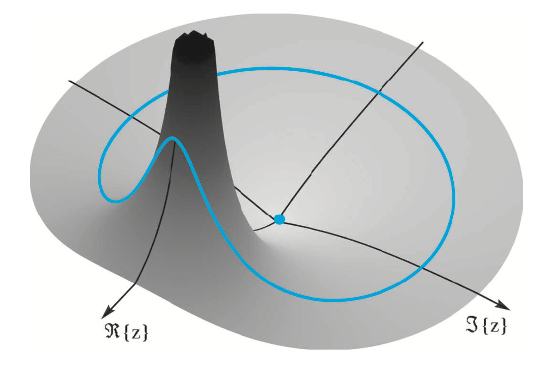
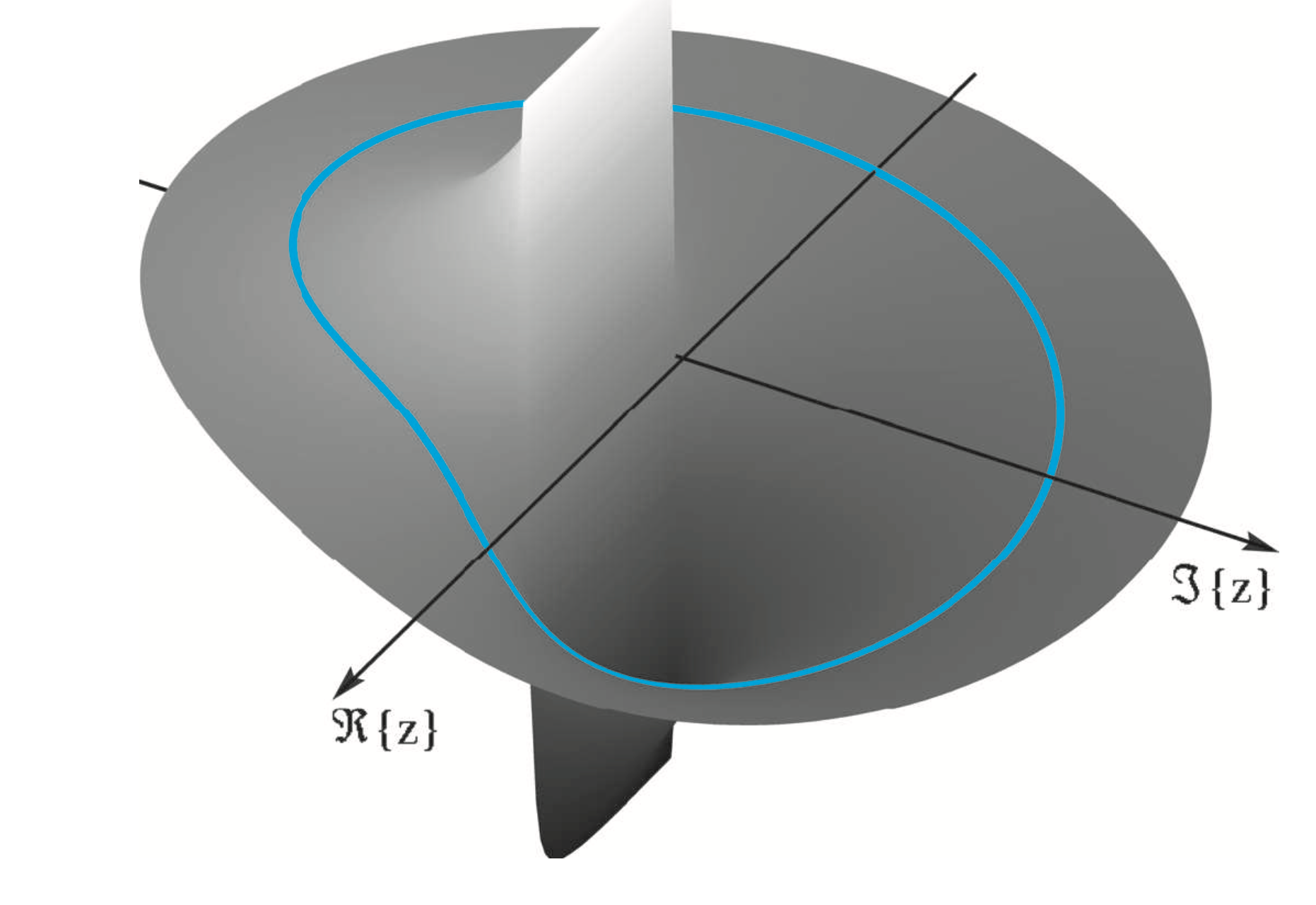
Three-Dimensional Plot of a System Function
We'll show that Frequency Response \(H\left(e^{j \hat{\omega}}\right)\), though is defined around unit circle(since \(|e^{j \hat{\omega}}| = 1\)), but is influenced by position of poles and zeros.
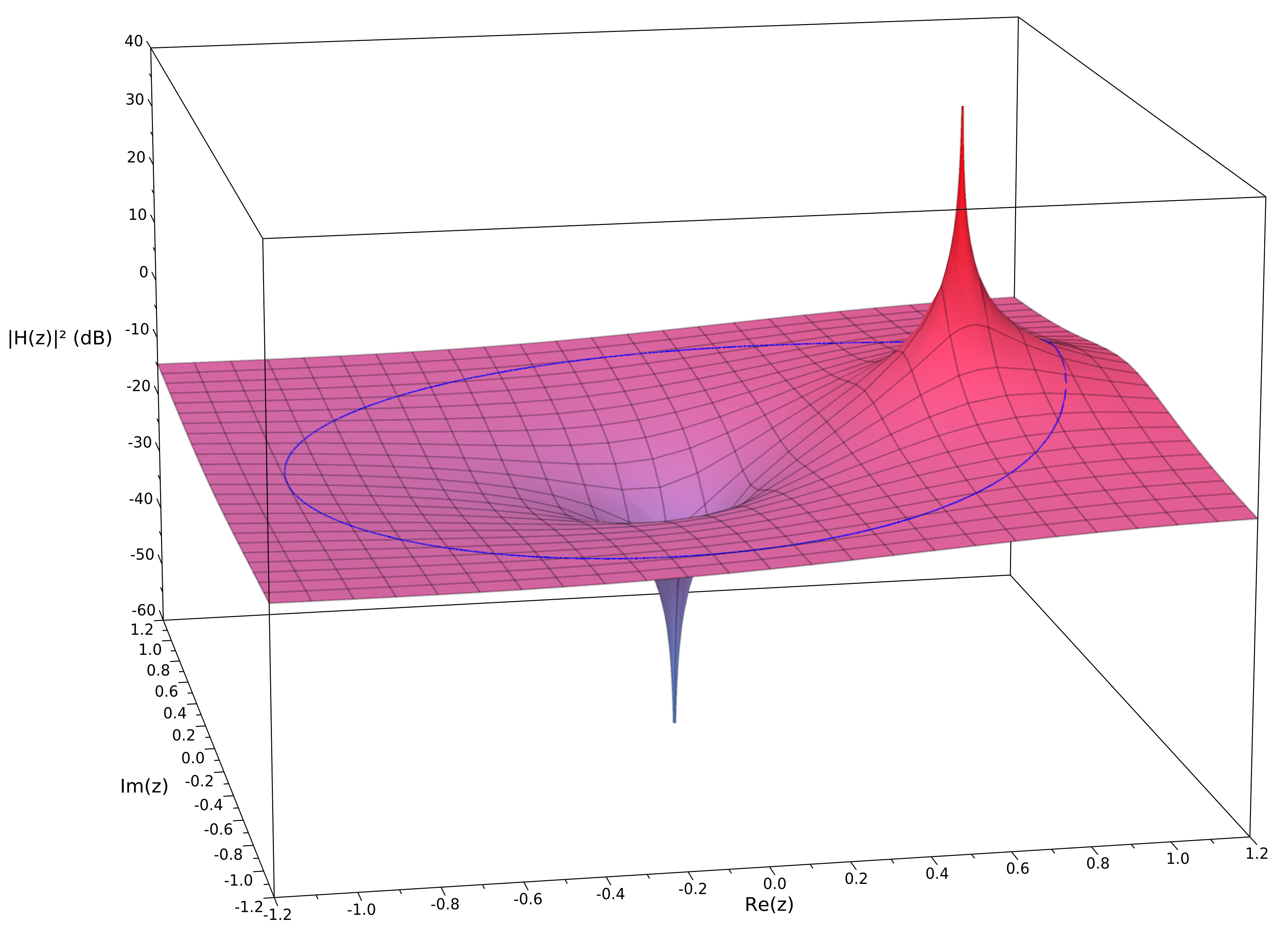
Image from: Pieter's blog.
The frequency response \(H\left(e^{j \hat{\omega}}\right)\) is obtained by selecting the values of \(H(z)\) only along the unit circle, because \(z=e^{j \hat{\omega}}\) defines the unit circle for \(-\pi<\hat{\omega} \leq \pi\).
We'll use the following example system function: \[ H(z)=\frac{1}{1-0.8 z^{-1}} . \] with a pole at \(z=0.8\) and a zero at \(z=0\).
Figures 10-10 and 10-11 are plots of the magnitude and phase of \(H(z)\) over the region \(|z| \leq 1.4\) of the \(z\)-plane.
Magnitude Response Plot
Figure 10-10 Magnitude of \(H(z)\) in (10.44) evaluated over a region of the \(z\)-plane including the unit circle. The first-order filter has a pole at \(z=0.8\) and a zero at \(z=0\) (shown with an orange dot). Values of \(|H(z)|\) along the unit circle are shown as a solid orange line where the frequency response (magnitude) is evaluated. The view is from the first quadrant, so the point \(z=1\) is in the foreground on the left.
In the magnitude plot of Fig. 10-10, we observe that the pole (at \(z=0.8\) ) creates a large peak that makes all nearby values very large. At the precise location of the pole, \(H(z) \rightarrow \infty\) !
(But the 3 -D surface has been truncated vertically, so the plot stays within a finite vertical scale.)
Phase Response Plot
The phase response in Fig. 10-11 also exhibits its most rapid transition at \(\hat{\omega}=0\) which is the point \(z=1\) (the closest point on the unit circle to the pole at \(z=0.8\) ).
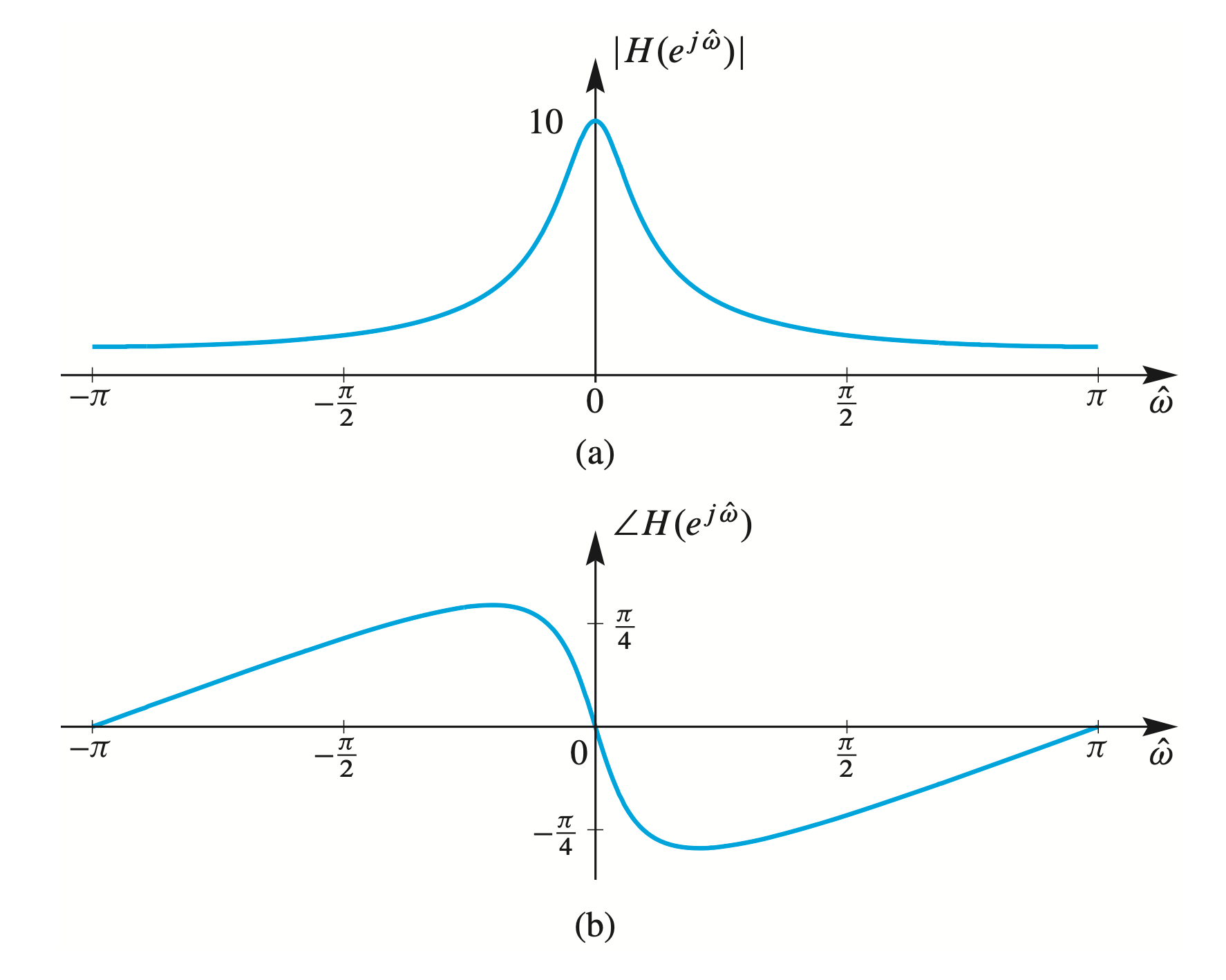
Two-dimensional Plots
Two-dimensional plots of \(H\left(e^{j \hat{\omega}}\right)\) versus \(\hat{\omega}\) are given in Fig. 10-12. The shape of the frequency response can be explained in terms of the pole location by recognizing that in Fig. \(10-10\) the pole at \(z=0.8\) pushes \(H\left(e^{j \hat{\omega}}\right)\) up in the region near \(\hat{\omega}=0\), which is the same as the point \(z=1\). The unit circle values follow the ups and downs of \(H(z)\) as \(\hat{\omega}\) goes from \(-\pi\) to \(+\pi\).
Figure 10-12: Frequency response for the first-order IIR filter (10.44). (a) Magnitude. (b) Phase.
The pole is at \(z=0.8\) and the numerator has a zero at \(z=0\). These are the values of \(H(z)\) along the unit circle in the \(z\)-plane of Figs. 10-10 and 10-11.
Three Domains
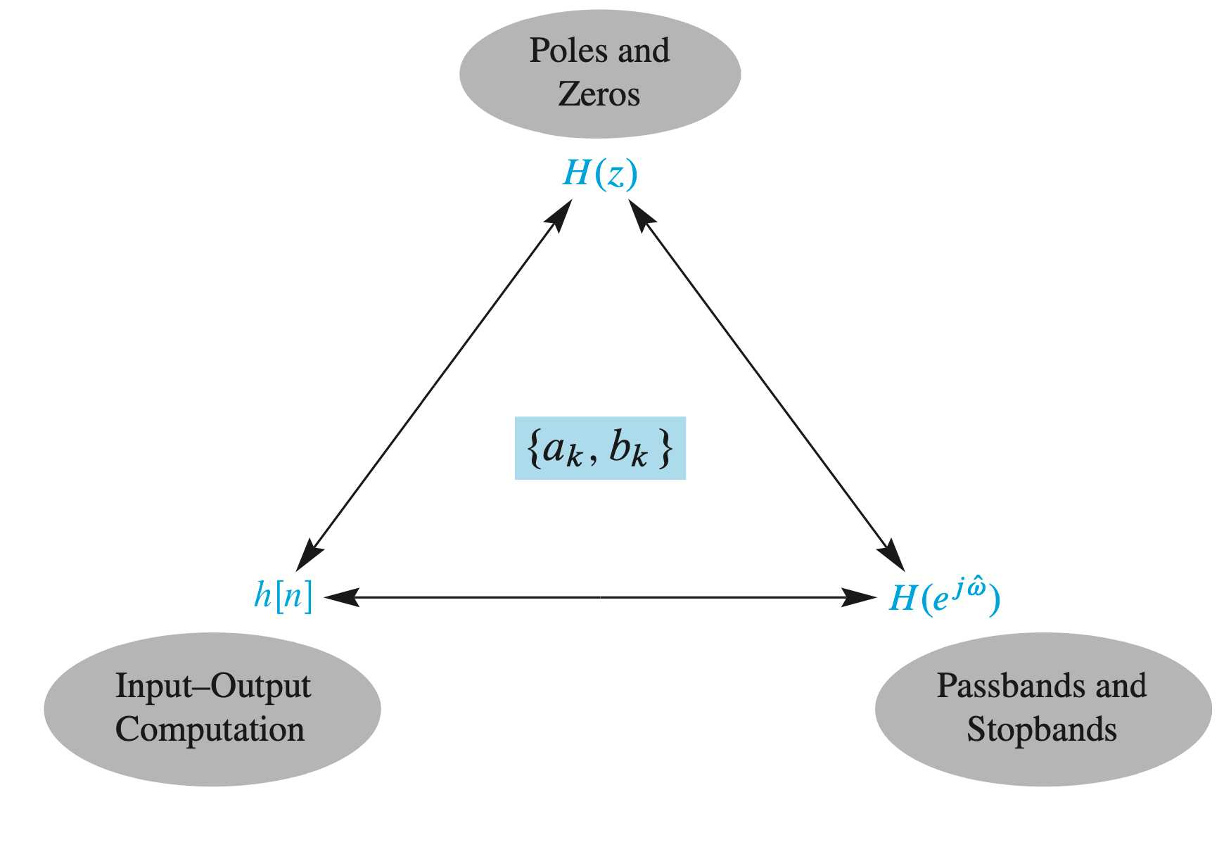
For example, consider an IIR filter with following feedback difference equation \[ y[n]=a_1 y[n-1]+a_2 y[n-2]+b_0 x[n]+b_1 x[n-1]+b_2 x[n-2] \] where coefficients \(\left\{a_1, a_2, b_0, b_1, b_2\right\}\) are constant.
The output is the impulse response \(h[n]\) when the input is \(x[n]=\delta[n]\).
In \(z\)-domain, this IIR filter is represented as \[ H(z)=\frac{b_0+b_1 z^{-1}+b_2 z^{-2}}{1-a_1 z^{-1}-a_2 z^{-2}} . \] And when the poles are inside the unit circle, we can obtain the frequency response, or the DTFT, by evaluating on the unit circle (\(z=e^{j \hat{\omega}}\)). \[ H\left(e^{j \hat{\omega}}\right)=\frac{b_0+b_1 e^{-j \hat{\omega}}+b_2 e^{-j 2 \hat{\omega}}}{1-a_1 e^{-j \hat{\omega}}-a_2 e^{-j 2 \hat{\omega}}} \]
Since \(H(z)\) is a ratio of polynomials, either the coefficients \(\left\{a_k, b_k\right\}\) or the poles and zeros of \(H(z)\) comprise a small set of parameters that completely define the filter.
FIR vs. IIR
- Zero poles = FIR
- Nonzero pole = IIR