Neural Networks
Sources:
- The spelled-out intro to neural networks and backpropagation: building micrograd
- Stanford CS231N, Lecture 4
Other useful resources:
StatQuest's Neural Networks videos
Efficient backprop. You need do download it via
1
wget http://yann.lecun.com/exdb/publis/pdf/lecun-98b.pdf
The python script and jupyter notebook used in this article can be found at here.
This article is a step-by-step explanation of neural networks which are extensively used in machine learning. It only involves the most basic case where the input of a neuron is a vector (1-D tensor)and output of a neuron is a scalar (0-D tensor). But the idea holds for higher, please reter to Derivatives, Backpropagation, and Vectorization for details.
# TODO
Notations
In this article we'll use following notations.
The gradient of a multivariate function \(f\) is a vector that contains all the partial derivatives of \(f\) with respect to each of its variables. Suppose \(f = f(x, y, z, \ldots)\), then the gradient would be a vector \(\left[\frac{\partial f}{\partial x}, \frac{\partial f}{\partial y}, \frac{\partial f}{\partial z}, \ldots\right]^T\), where each component is the partial derivative of \(f\) with respect to one of its variables.
However, I'll also call the partial derivative of a function, denoted as \(\frac {\partial f} {\partial w}\), where \(f\) is a multivariable function and \(w\) is a variable of \(f\), as a gradient, denoted as \(\nabla_w f\).
To sum, the terms "gradient" and the "derivative" or "partial derivative" are all interchangeable in this article.
We refer gradient to gradient formula. It's different from the gradient value, which is a value of the gradient).
- A gradient formula is a vector of partial derivative formulars.
- A gradient value is a vector of partial derivative values.
- A gradient value is evaluated from the gradient formula.
NN is short for a neural network.
FP is short for forward pass, or foreward propagation.
BP is short for backward pass, backward propagation or backpropagation.
Article organization
The math model of neural network is computational graph, every operation of NN, including FP, BP and other fancy operations (like stop gradient in PyTorch) can be intuitively implemented and visualized on computational graph.
Thus, in this article, we take a view of computational graph to understand neural network. The organization is as follows:
To prepare, we first introduce the basic concepts of gradient.
We start from defining the
Valueclass, aValueobject is represent a single node in computational graph. Our implementation is highly similar to PyTorch'sTensorclass.Next, we illustrate the idea of back propagation and how to back propagate through the total graph.
In addition, since back propagation depends on concrete computation operations, we then introduce how to define each operation and let it support BP.
Now we know the idea of back propagation and support it in
Valueclass. We use the later to build the components of neural networls, i.e.,- We build a neoron first.
- Then we use neuron to build a linear layer.
- At last, we organize layers to form a multilayer perceptron (MLP).
Finally, we know FP, BP, how a NN is organized. We then show how to train this NN. We also orgainze our NN in a more modular way: letting all components inherit from a
Moduleclass.
Basic concepts
Neural networks
A neoral network (NN) is a function that maps input data to output data. For example, given a dataset with \(n\) data points (or samples) \((x_1, y_{1}), \dots, (x_n, y_n)\), the neural network acts as a function, say \(f\), that expressing the "relationship" between \(x\) and \(y\): \[ f_\theta: X \rightarrow \hat Y, \] where
- \(X, Y, \hat Y\) are the sets of all \(x_i, y_i, \hat y_i\), \(i \in \{1,2,\cdots, n \}\).
- \(\hat y_i\) is the output value of the NN corresponding to input data \(x_i\).
- \(y_i\) is the value in the dataset corresponding to data \(x_i\).
- \(\theta\) is the set of all parameters of the NN. The parameters are all weights and biases.
Loss function
The goal of a neural network is to minimize the value of a loss function \[ \text{Loss}(y, \hat y) = \cdots . \] Since the loss function, the architecture of the NN, and the dataset are all given. What we can do is modifying (or optimizing) its parameters \(\theta\). The optimization process is called training the NN.
Derivative
Given a function \(f(x) = 3x^2 - 4x + 5\),
1 | def f(x): |
It has plot:
1 | xs = np.arange(-5,5, 0.25) |
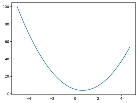
The derivative equation of function \(f\) w.r.t. variable \(x\) is \[ \begin{equation} \label{derivative} f^\prime(x) = \frac {\partial f} {\partial x}=\lim _{h \rightarrow 0} \frac{f(x+h)-f(x)}{h} . \end{equation} \] In this example, the derivative equation of \(f(x)\) w.r.t. variable \(x\) is \(6x-4\). When \(x=2/3\), the derivative becomes \(0\).
The physical meaning of \(\frac {\partial f} {\partial x}\) is that "when \(x\) changes a little bit, how much will \(f\) change".
You can test it:
1 | hs = np.arange(0.0001,0.0, -0.00001) |
The output is:
1 | h=0.0001, value=0.0002999999981767587 |
As \(h\) decreases, the value approaches \(0\), which is the derivative value \(f^\prime(2/3) = 0\).
Help functions
For better understanding, we use these functions to visualize our computational graph:
1 | def trace(root): |
Value class
Now we implement a basic Value class which shares the most fundamental features of Tensor in PyTorch.
1 | class Value: |
Each Value object is a node in the computational graph. If it's computed via an operation, such as __add__, __mul__, __neg__, __true_div__ (not defined yet), it should set it's the operand(s) generating it as its predessor(s). This predecessorr relationship is implemented by the self._prev in each Value object.
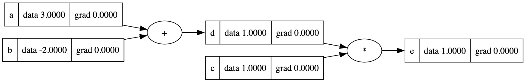
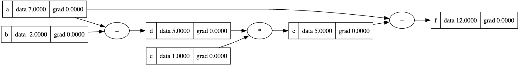
1 | a = Value(3, label='a') |
The visualized computational graph is:

For now we haven't implement the gradient computation yet, so in the previous graph each node doesn't have a gradient value. Let's see how gradient calculation is implemented in the computational graph.
Gradient of each node
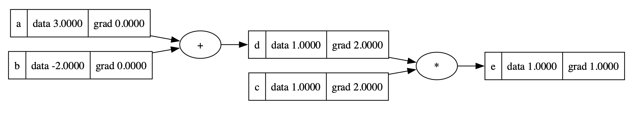
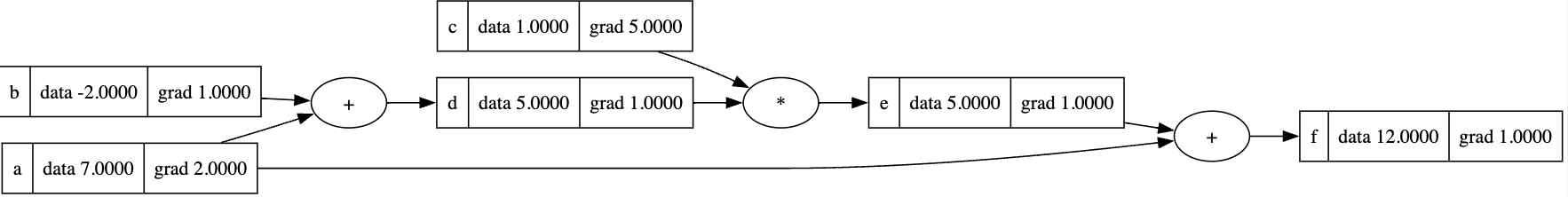
Now let's see the gradient value of each variable. We define a function \(L = (ab+c)f\), and compute its gradient value with respect to variable a, b, c, etc.
1 | def lol(): |
We set h=0.001. When we add h to b, the value of (L2 - L1)/h is -3.99999999.... If we continue to decrease h, we'll find that the value approaches 4.0, which is exactly the gradient value \[
\frac {\partial L} {\partial b}|_{b=-3.0} = af,
\] since a=2.0, f=-2.0, \(\frac {\partial L} {\partial b}|_{b=-3.0} = -4.0\).
Backpropagation
The idea of backpropagation
We now know that given a function \(L\) and a variable \(x\), we can calculate the gradient via equation \(\eqref{derivative}\). However, a more efficient way is to leverage the chain rule in Calculous: \[ \frac{d z}{d x}=\frac{d z}{d y} \cdot \frac{d y}{d x} . \] The intuition here is that, given a function \(L(x,y,z) = (x+y) z\), let \(u = x+y\), then this function transforms to \(L(u,z) = uz\), for computing the gradient of \(x,z\), we can calculate \(\frac{df}{d u} = z\) first, then leverage the chain rule to calculate
\[
\begin{align}
\frac{d L}{d x}=\frac{d L}{d u} \cdot \frac{d u}{d x} \label{chain_rule}\\
\frac{d L}{d y}=\frac{d L}{d u} \cdot \frac{d u}{d y} \nonumber .
\end{align}
\] The gradient that have been already computed, i.e., \(\frac{d L}{d u}\) in equation \(\eqref{chain_rule}\), is called the upstream gradient of node x or y, since it's to be multiplied with the local gradient \(\frac{d u}{d x}\) or \(\frac{d u}{d y}\).
The gradient of x or y is local gradient * upstream gradient.
In summary:
- The upstream gradient of node \(x\) or \(y\): \(\frac{d L}{d u}\).
- The local gradient of node \(x\) or \(y\): \([\frac {\partial u} {x}, \frac {\partial u} {y}]^T\)
- The gradient of node \(x\) or \(y\): \([\frac {\partial L} {x}, \frac {\partial L} {y}]^T\).
In order to leverage chain rule, we must do derivation of the computational graph in a backward manner. In other words, we must calculate \(\frac{d L}{d u}\) before calculating \(\frac{d u}{d x}\) and \(\frac{d u}{d y}\).
In this sense, the derivation process is called back(ward) propagation.
- A detailed illustration is --> here.
One thing to notify is that the derivative of a variable with respect to itself is 1, i.e., for variable \(y\), \[
\frac{d}{d y} y=1 .
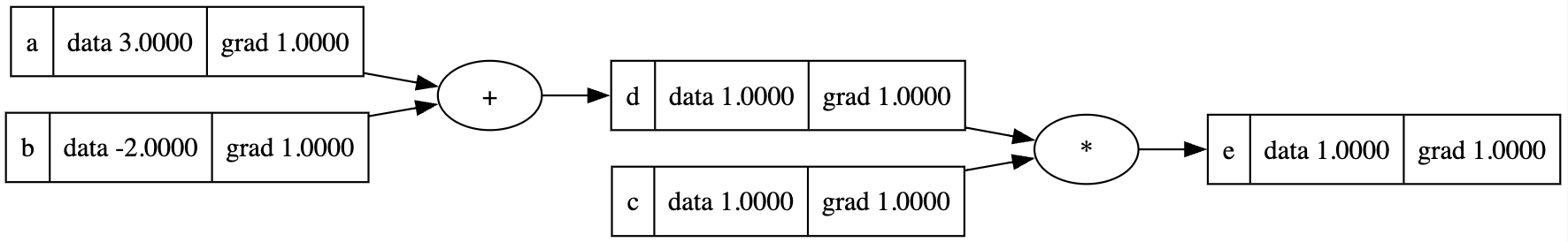
\] Take the e node in the previous section as an example, we have function \(L = (a+b)c\) and variable \(e = (a+b)c\), thus \(\frac {\partial L} {\partial e} = \frac {\partial e} {\partial e} = 1\).
So we set the last node of the computational graph to have gradient=1.0 (you can think it as local gradient=1.0 and there's no upstream gradient).
We implement this in python by:
- Add
gradattribute toValueobject. - For each computation operation, such as add, multiplication, division (not defined yet), etc, we implement the back propagate process as
_backwardmethod.
1 | class Value: |
Each operation node Recall that in computational graphs, a node is a function. During backward propagation, w
corresponds to a "local gradient", that
For instance, the multiplication operation \(L=ab\) has gradient \(\frac {\partial L} {\partial a}= b, \frac {\partial L} {\partial b}= a\), so the
1 | a = Value(3, label='a') |
We backpropagate through node e:
1 | e.grad = 1.0 # The last node should have gradient = 1.0 |
The gradient of node d is 1.0, which equals to the value of node c; the gradient of node c is 1.0, which equals to the value of node d.
Moreover, the addition operation \(L=a+b\) has gradient \(\frac {\partial L} {\partial a}= 1, \frac {\partial L} {\partial b}= 1\), so that we backpropagate through node d
1 | d._backward() |
To back progapate the whole computational graph, we need to call backward() for each node (if we can) mannually.
1 | e.backward() |
In this section, we defined the _backward method for operations __add__ and __mul__. It can be implied that we can define the _backward method for whatever operation we want to compute it's gradient as long as it's feasible, i.e., the operation itself is first-order differentiable.
However, we must call the _backward method for each node manually in some fixed order, we can't back propagate c before back propagate e. Is there any way to automate this process so that we can do back propagation only once and calculate the gradient for the whole graph?
Backpropagate through the whole graph
The solution is simple:
- Remember that the last node itself must set its gradient to 1.0.
- Sort all the nodes in the computational graph in a topological order.
- From the last node to the first node in the computational graph, call their
_backwardmethod seperately.
Here's the code:
1 | class Value: |
We can call this backward method to the last node of any computational graph without the heavy manual work.
1 | a = Value(7, label='a') |
1 | f.grad = 1.0 |
Operations to be back propagated
Now we define more commonly used operations and add _backward support to them.
Operations can be set on arbitary abstraction level
Note that the operation can be set at arbitary abstraction level.
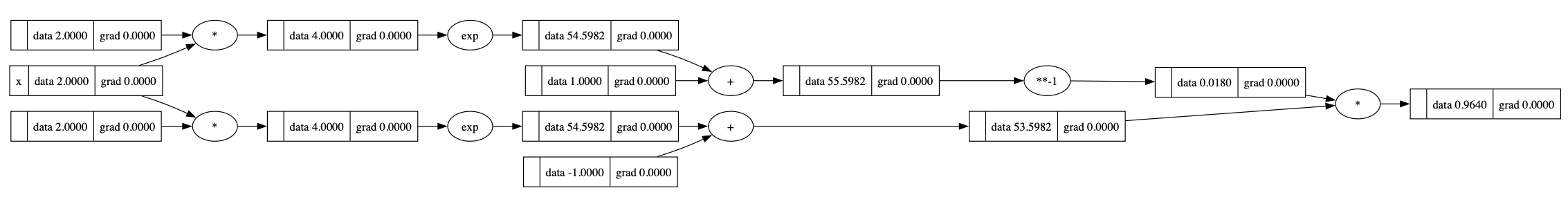
For example, for tanh function: \[
\begin{aligned}
\tanh (x)=\frac{e^{2 x}-1}{e^{2 x}+1}
\end{aligned}
\] with derivative \[
\frac{d}{d x} \tanh (x)=1-\tanh (x)^2 =1-\frac{\left(e^x-e^{-x}\right)^2}{\left(e^x+e^{-x}\right)^2} .
\] We can either define tanh outside of Value class, and define operations divisiontogether with exponent.
Low level
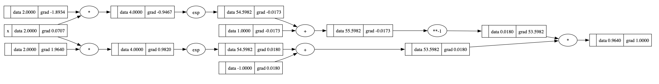
We can build tahh from low level through defining exp, addition and other low level operations. We don't have to define tanh in the Value class.
1 | class Value: |
Create the graph:
1 | def tanh(x): |
Start back propagation:
1 | o.grad = 1.0 |
High livel
We can define the _backward for tanh instead:
1 | class Value: |
Cteate the graph:
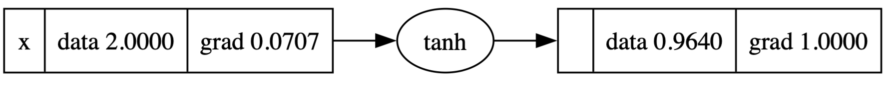
1 | x = Value(2.0, label='x') |

Start back propagation:
1 | o.grad = 1.0 |
Operation zoo
Addition
\[ \begin{aligned} \frac{d}{d x}\left(x+y\right) = 1 \\ \frac{d}{d y}\left(x+y\right) = 1 \end{aligned} \]
1 | def __add__(self, other): |
Multiplication
\[ \begin{aligned} \frac{d}{d x}\left(xy\right) = y \\ \frac{d}{d y}\left(xy\right) = x \end{aligned} \]
1 | def __mul__(self, other): |
Negation
We achieve negation through multiplication: \[ -x = x \cdot (-1) . \]
1 | def __neg__(self): # -self |
Substraction
We achieve substraction through addition and negation: \[ x - y = x + (-y) \]
1 | def __sub__(self, other): # self - other |
Exponential function
\[ \frac{d}{d x}\left(e^x\right) = e^x . \]
So the local graddient is just the data of the output.
1 | def exp(self): |
Power
\[ \frac{d}{d x} \left(x^n\right) = n x^{n-1} . \]
1 | def __pow__(self, other): |
Division
We achieve division through power: \[ x / y = x \cdot y^{-1} . \]
1 | def __truediv__(self, other): # self / other |
tanh
As before, tanh is
1 | def tanh(self): |
Relu
The derivative of relu at x=0 is set to 0.
1 | def relu(self): |
Neuron
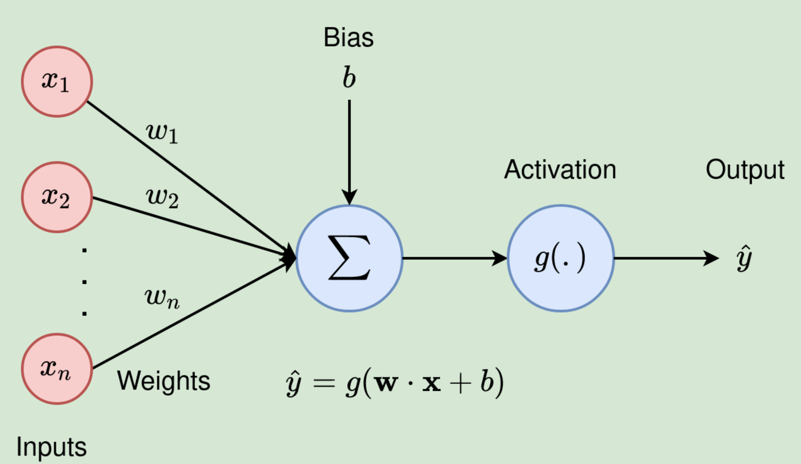
--> Image source
Now we know backpaopagation, it's time to investigate Neural networks. In this section, we are going to implement a single neuron conducting computation \[ \hat y = g(\sum_{i=1}^{n} w_i x_i + b) \] where the input is a vector \(x\) with length \(n\), the output is a scalar \(y\), the activation function is denoted as \(g\), the parameters can be solit into two parts:
- A weight vector \(w\), should have length \(n\) as well.
- A bias \(b\), which is a scaler.
We also implement the parameters method to get all the \(n+1\) parameters of this neuron, i.e., the \(n\) weights and one bias.
1 | class Neuron(): |
The compututational graph of a neuron is like:
1 | x = [2.0, 3.0, -1.0] |
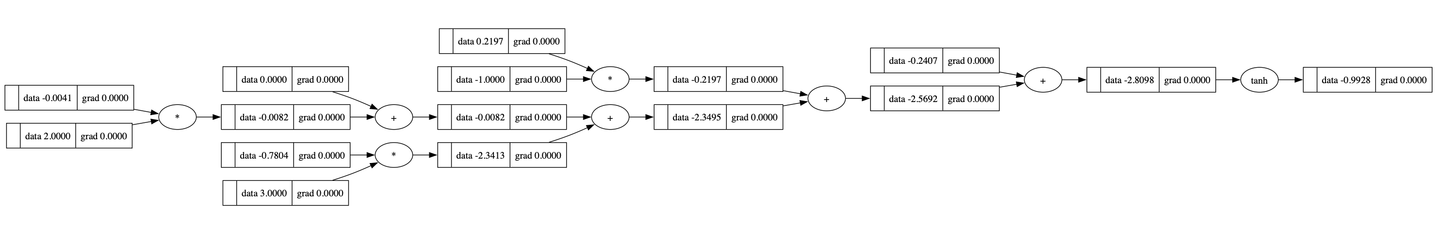
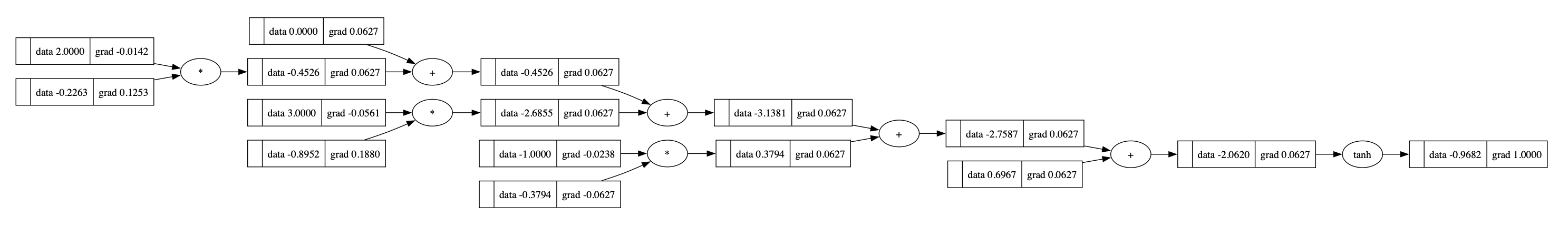
We can backpropagate it:
1 | o.backward() |
Layer
In the same way, we define a layer (or linear layer since every neuron performs linear transformation):
1 | class Layer(): |
Basically, each neuron (only its weights part) is like a colum vector in the matrix. For example, a layer with 200 neurons, each neuron takes a 30-D input looks like:
1 | # Pseudo code of a linear layer |
Multilayer perceptron
Referrence: Using neural nets to recognize handwritten digits
Despite it's fancy name, a multilayer perceptron (MLP) is just a combination of linear layers, it'sorganized in at least three layers:
- Input Layer
- Hidden Layer(s)
- Output Layer
Below is a simple MLP with one input layer (dimension=3), two hidden layers (dimension=4 for each), one output layer (dimension=1):
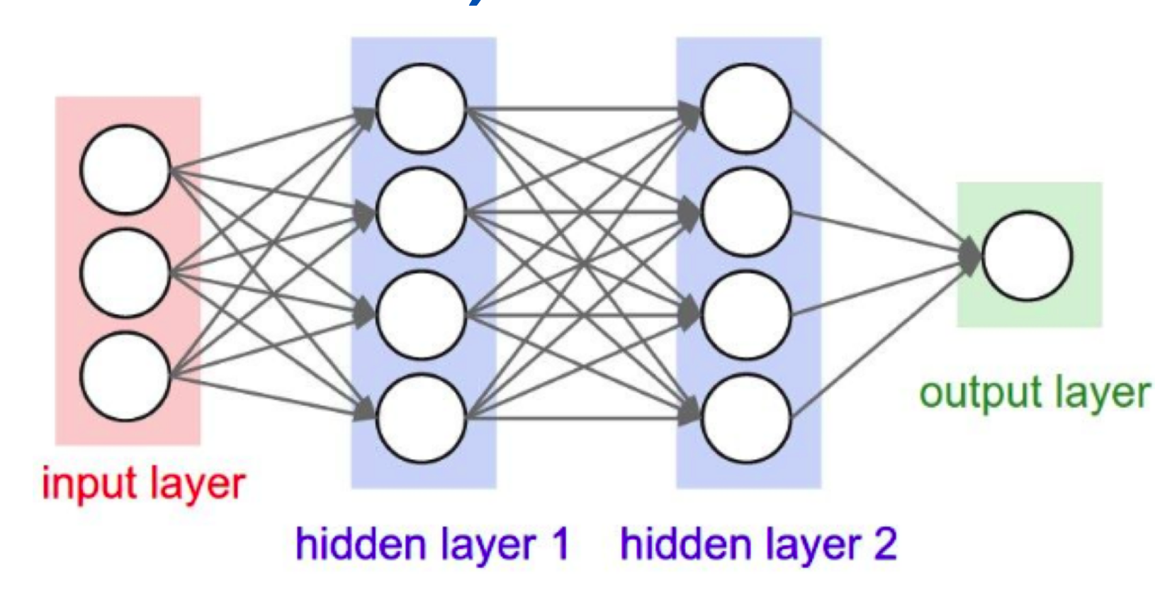
Incidentally, when I defined perceptrons I said that a perceptron has just a single output. In the network above the perceptrons look like they have multiple outputs. In fact, they're still single output. The multiple output arrows are merely a useful way of indicating that the output from a perceptron is being used as the input to several other perceptrons. It's less unwieldy than drawing a single output line which then splits.
1 | class MLP(): |
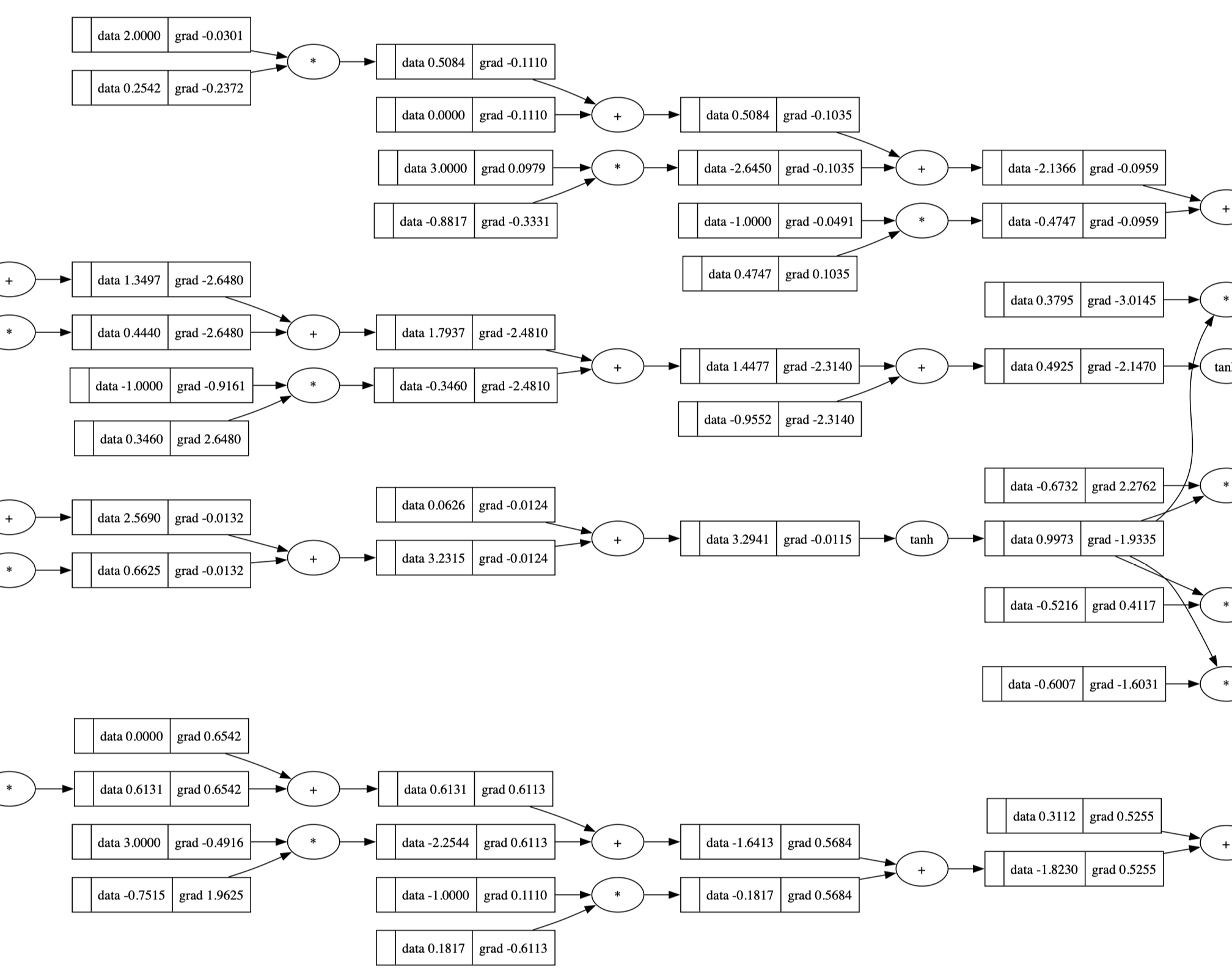
Now we create the computational graph for MLP:
1 | x = [2.0, 3.0, -1.0] |
Note that the graph has already been very huge:
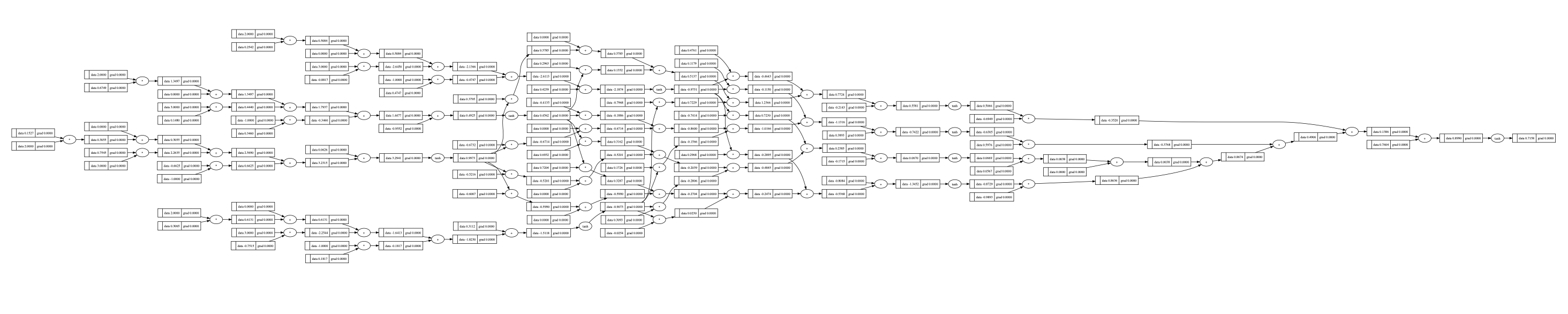
As before, we can easily back propagate it:
1 | o.backward() |
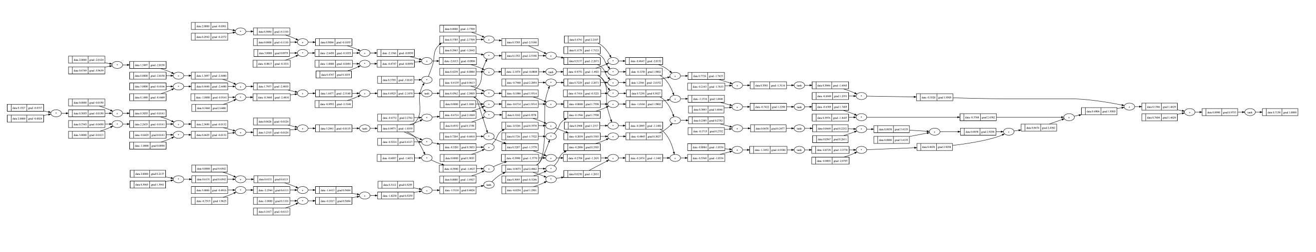
One glimpse into it:
Pseudo code for a MLP:
1 | # Here we define a MLP with two layers. The MLP takes a 30-D input and produces a 27-D output. |
Training process
1 | def train(n, episodes=20, learning_rate=-0.1): |
During each training iteration, we do forward pass and backward pass, then use the gradient to update the parameters.
1 | if __name__ == '__main__': |
Output:
1 | 0 3.0023652813181076 |
We must flash the gradients before doing BP. Otherwise the gradients in each iteration will accumulate. This can be implemented as a function zero_grad, which is what PyTorch did.
Module
At last, to be more compatible with PyTorch, we organize our NN, let all componnets (Neuron, Layer and MLP) inherit a base Module class:
1 | class Module: |