Data Compression

Ref:

1. EE 376A: Information Theory. Winter 2018. Lecture 6. - Stanford University
2. EE 376A: Information Theory. Winter 2017. Lecture 4. - Stanford University
3. Elements of Information Theory

Notations

• rv: random variable.
• Let $x^n$ denote $(x_1,x_2,\dots ,x_n)$.

Codes

• Definition: A source code $C$ for a random variable $X$ is a mapping from $\mathcal{X}$, the range of $X$, to ${\mathcal{D}}^{\ast }$, the set of finite-length strings of symbols from a $D$-ary alphabet. Let $C(x)$ denote the codeword corresponding to $x$ and let $l(x)$ denote the length of $C(x)$.

  • That is, a code $C$ of rv $X$ is a function from $\mathcal{X}$ to ${\mathcal{D}}^{\ast }$.
  • For example, $C($ red $)=00,C($ blue $)=11$ is a source code for $\mathcal{X}=\{$ red, blue $\}$ with alphabet $\mathcal{D}=\{0,1\}$.

• Definition: The expected length $L(C)$ of a source code $C(x)$ for a random variable $X$ with probability mass function $p(x)$ is given by $$L(C)=\mathbb{E}(l(x))=\sum _{x\in \mathcal{X}}p(x)l(x)$$ where $l(x)$ is the length of the codeword associated with $x$.

• Definition: The extension $C^{\ast }$ of a code $C$ is a function of stochastic process $X^n$. $$C^{\ast }(x^n)=C\left(x_1\right)C\left(x_2\right)\cdots C\left(x_n\right),$$ where $C\left(x_1\right)C\left(x_2\right)\cdots C\left(x_n\right)$ indicates concatenation of the corresponding codewords.

  • Example: If $C\left(x_1\right)=00$ and $C\left(x_2\right)=11$, then $C\left(x_1{x}_2\right)=0011$.
  • Note: For convience, we'll use the notation $C(x^n)$ instead of $C^{\ast }(x^n)$.

Example

Without loss of generality, we can assume that the $D$-ary alphabet is $\mathcal{D}=\{0,1,\dots ,D-1\}$.

Let $X$ be a rv with the following distribution and codeword assignment: $$\begin{array}{ll}\mathrm{Pr}(X=1)=\frac{1}{2},& \text{ codeword }C(1)=0\\ \mathrm{Pr}(X=2)=\frac{1}{4},& \text{ codeword }C(2)=10\\ \mathrm{Pr}(X=3)=\frac{1}{8},& \text{ codeword }C(3)=110\\ \mathrm{Pr}(X=4)=\frac{1}{8},& \text{ codeword }C(4)=111.\end{array}$$

The entropy $H(X)$ of $X$ is 1.75 bits: $$\begin{array}{rl}H(X)& =\mathbb{E}(l(x))\\ & =p(X=1)\log \frac{1}{p(X=1)}+p(X=2)\log \frac{1}{p(X=2)}+p(X=3)\log \frac{1}{p(X=3)}+p(X=4)\log \frac{1}{p(X=4)}\\ & =(1/2\cdot 1)+(1/4\cdot 2)+(1/8\cdot 3)+(1/8\cdot 3)\\ & =1.75\end{array}$$

The expected length $L(C)=\mathbb{E}(l(x))$ of this code is also 1.75 bits: $$\begin{array}{rl}L(C)& =\mathbb{E}(l(x))\\ & =p(X=1)l(X=1)+p(X=2)l(X=2)+p(X=3)l(X=3)+p(X=4)l(X=4)\\ & =(1\cdot 1/2)+(2\cdot 1/4)+(3\cdot 1/8)+(3\cdot 1/8)\\ & =1.75\end{array}$$

Here we have a code that has the same average length as the entropy. We note that any sequence of bits can be uniquely decoded into a sequence of symbols of $X$. For example, the bit string 0110111100110 is decoded as 134213.

Classes of Codes

Classes of Codes

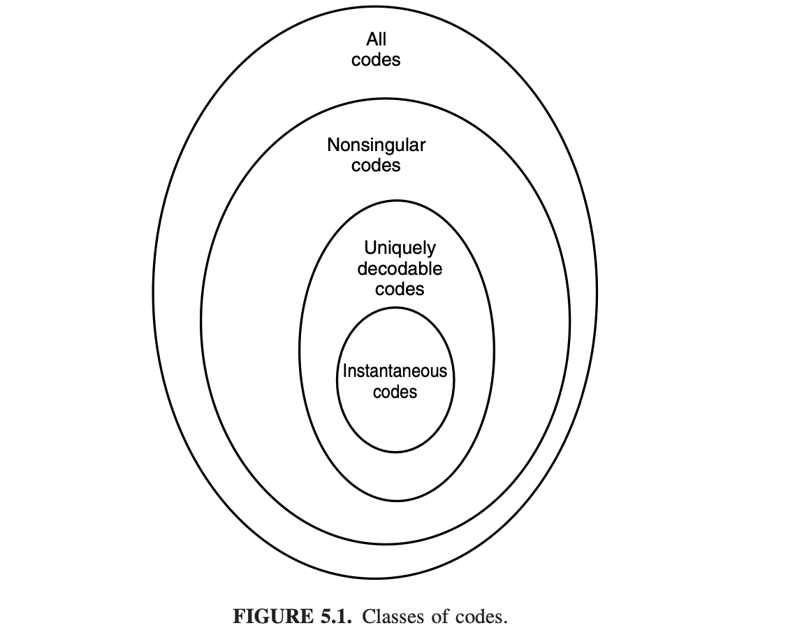
Nonsingular Codes

Definition: A code is said to be nonsingular if it's an injection; i.e., every element of the range of $X$ maps into a different string in ${\mathcal{D}}^{\ast }$. $$x\ne x^{\prime }\Rightarrow C(x)\ne C\left(x^{\prime }\right).$$

Nonsingularity suffices for an unambiguous description of a single value of $X$.

But we usually wish to send a sequence of values of $X$. In such cases we can ensure decodability by adding a special symbol (a "comma") between any two codewords.

But this is an inefficient use of the special symbol; we can do better by developing the idea of self-punctuating or instantaneous codes.

Uniquely Decodable

Definition: A code is called uniquely decodable if its extension is an injection(nonsingular); i.e, every element of the range of $X^n$ maps into a different string.

However, one may have to look at the entire string to determine even the first symbol in the corresponding source string.

Prefix Codes

Definition: A code is called a prefix code or an instantaneous code if no codeword is a prefix of any other codeword.

• A prefix code is uniquely decodable and self-punctuating(i.e. without needing entire binary sequence before decoding starts)

Example

To illustrate the differences between the various kinds of codes, consider the examples of codeword assignments $C(x)$ to $x\in \mathcal{X}$ in following table:

$X$	Singular	Nonsingular, But Not Uniquely Decodable	Uniquely Decodable But Not Instantaneous	Instantaneous
1	0	0	10	0
2	0	010	00	10
3	0	01	11	110
4	0	10	110	111

1. For the nonsingular code, the code string 010 has three possible source sequences:

   1. 2
   2. 14
   3. 31

   and hence the code is not uniquely decodable.

2. For the uniquely decodable code but not prefix-free code:

   1. If the first two bits are 00 or 10, they can be decoded immediately.
   2. If the first two bits are 11, we must look at the following bits.
      1. If the next bit is a 1, the first source symbol is a 3.
      2. If the length of the string of 0’s immediately following the 11 is odd, the first codeword must be 110 and the first source symbol must be 4;
      3. if the length of the string of 0’s is even, the first source symbol is a 3.

   By repeating this argument, we can see that this code is uniquely decodable. Sardinas and Patterson [455] have devised a finite test for unique decodability, which involves forming sets of possible suffixes to the codewords and eliminating them systematically.

3. The fact that the last code in Table 5.1 is instantaneous is obvious since no codeword is a prefix of any other.

Kraft-McMillan Inequality

Theorem: (Kraft-McMillan Inequality). For all D-ary uniquely decodable (UD) codes:

$$\begin{array}{}\text{(1)}& \sum _{x\in \mathcal{X}}{D}^{-l(x)}\le 1\end{array}$$

Converse: any integer-valued function satisfying this inequality is the length function of some UD code.

• Note since every prefix code is uniquely decodable, this inequality also holds for prefix codes.

• Sometimes this equation is written as $\sum D^{-l_i}\le 1$.

Proof

Take any uniquely decodable code and let $l_{max}=maxl(x)$. Fix any integer $k$ and observe: $$\begin{array}{rl}{\left(\sum _{x\in \mathcal{X}}{D}^{-l(x)}\right)}^k& =\left(\sum _{x_1}{D}^{-l\left(x_1\right)}\right)\cdot \left(\sum _{x_2}{D}^{-l\left(x_2\right)}\right)\cdot \dots \cdot \left(\sum _{x_k}{D}^{-l\left(x_k\right)}\right)\\ & =\sum _{x_1}\sum _{x_2}\dots \sum _{x_k}\prod _{i=1}^k{D}^{-l\left(x_i\right)}\\ & =\sum _{x_1,\dots x_k}{D}^{-\sum _{i=1}^{k}l\left(x_i\right)}\\ & =\sum _{x^k\in {\mathcal{X}}^k}{D}^{-l\left(x^k\right)}\\ & =\sum _{m=1}^{k\cdot l_{max}}a(m)\cdot D^{-m}\end{array}$$

Explain:

• The transition from 1st to 2nd line is that we just assign index 1,2,...,k to $x$. //TODO
• $l(x^k)$ is the length of the string/sequence $x^k$(or $x_1,x_2,\cdots ,x_k$).
• $a(m)$ is the number of source sequences xk mapping into codewords of length $m$.

Since the code is uniquely decodable, the mapping is one-to-one, so:

1. there is at most one sorce symbol sequence mapping into each code $m$-length codeword sequence
2. and there are at most $D^m$ code $m$-length codeword sequence.

Thus, $a(m)\le D^m$, and we have $$\sum _{m=1}^{k\cdot l_{max}}a(m)\cdot D^{-m}\le \sum _{m=1}^{k\cdot l_{max}}{D}^m\cdot D^{-m}=k{l}_{max}.$$

So we can get an upper-bound: $${\left(\sum _{x\in \mathcal{X}}{2}^{-l(x)}\right)}^k\le \sum _{m=1}^{k\cdot l_{max}}{D}^m\cdot D^{-m}=k\cdot l_{max}$$

Notice that the exponential term ${\left(\sum _{u\in \mathcal{U}}{2}^{-l(u)}\right)}^k$ is in fact upper-bounded by $k\cdot l_{\text{max }}$, which is linear in $k$.

From this we arrive at the theorem's claim (note that the inequality holds for all $k>0$ ): $$\sum _{x\in \mathcal{X}}{2}^{-l(x)}\le \underset{k\to \mathrm{\infty }}{lim}{(k\cdot l_{max})}^{1/k}=1$$

Proof of Converse

Construct prefix code

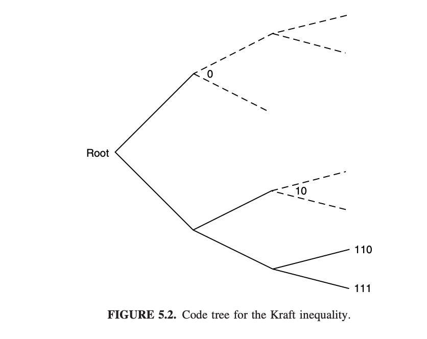
Proof of converse: given any set of $l_1,l_2,...,l_m$ satisfying the Kraft-McMillan Inequality, we can construct an prefix code as:

1. Consider a D-ary tree in which each node has D children. Let the branches of the tree represent the symbols of the codeword. Then each codeword is represented by a leaf on the tree. The path from the root traces out the symbols of the codeword.

   Note: no codeword is an ancestor of any other codeword on the tree. So that it's a prefix tree.

   Note: even for a "leaf", we continue to write its descendants.

2. Label the first node (lexicographically) of depth $l_1$ as codeword 1, and remove its descendants from the tree. Note: for $i\ne j$, $l_i$ may equal to $l_j$.

3. Then label the first remaining node of depth $l_2$ as codeword 2, and so on.

4. Proceeding this way, we construct a prefix code with the specified $l_1,l_2,...,l_m$.

Optimal Codes

An optimal code is a prefix code with the minimum expected length.

From the results of Kraft-McMillan Inequality, this is equivalent to finding the set of lengths $l_1,l_2,\dots ,l_m$ with minimum expected length while satisfying the Kraft-McMillan Inequality.

This is a standard optimization problem: Minimize $$L=\sum p_i{l}_i$$ over all integers $l_1,l_2,\dots ,l_m$ satisfying $$\sum D^{-l_i}\le 1$$

Bounds on the Optimal Code Length

Theorem: The expected length $L$ of any uniquely decodable (UD) D-ary code for a random variable $X$ is $$\begin{array}{}\text{(2)}& H_D(X)\le L\le H_D(X)+1\end{array}$$

Proof: $H_D(X)\le L$

Let $q(x)=c{2}^{-l(x)}$ be a P.M.F. where the normalizing constant $c$ is chosen such that the probability sums to 1 .

We knwo that $c\ge 1$.

Proof:

1. By the Kraft-McMillan Inequality $\text{(1)}$, $\sum _{x\in \mathcal{X}}{D}^{-l(x)}\le 1$.
2. Since $q(x)=c\cdot 2^{-l(x)}$, $c=\frac{1}{\sum _{x\in \mathcal{X}}{D}^{-l(x)}}$, so $c\ge 1.$

Next, consider the relative entropy between the probability distributions of the source $p$ and $q$ (Taking advantage of ): $$\begin{array}{rl}0& \le D(p\Vert q)\\ & =\sum _{x}p(x){\log }_D\frac{p(x)}{q(u)}\\ & =\sum _{x}p(x){\log }_{D}p(x)+\sum _{x}p(x){\log }_D\frac{1}{q(u)}\\ & =\sum _{x}p(x){\log }_{D}p(x)+\sum _{x}p(x)[l(u)-\underset{\ge 0}{\underbrace{{\log }_{D}c}}]\\ & \le -H(X)+L\end{array}$$

Explain:

• The first line is from the non-negativity of relative entropy.
• The last line is due to $H(X)=-\sum _{x}p(x)\log p(x)$ and $L=\sum _{x}p(x)l(u)$.
• ${\log }_{D}c\ge 0$ is from the fact that $c\ge 1$.

Note: Beyond its role in this proof, the relative entropy has significance in the context of compression. Suppose we have length function $l(u)\approx -\log q(u)$ for some P.M.F. $q$. This code will be near optimal if the source distribution is $q(u)$. However, if the true source distribution is $p(x)$, then, $$\begin{array}{rl}L-H_D(X)& \approx \mathbb{E}[{\log }_D\frac{1}{q(x)}]-\mathbb{E}[{\log }_D\frac{1}{p(x)}]\\ & =\sum _{x}p(x){\log }_D\frac{p(x)}{q(x)}\\ & =D(p\Vert q)\end{array}$$

The relative entropy can be thought of as the cost of mismatch in lossless compression, i.e. the expected number of excess bits that will be expended due to optimizing the code for distribution $q$ when the true distribution is $p$.

Proof: $L\le H_D(X)+1$

Recall the setup of Kraft-McMillan Inequality $\text{eqrefNaN}$: We wish to minimize $L=\sum _{-}{p}_i{l}_i$ subject to the constraint that $l_1,l_2,\dots ,l_m$ are integers and $\sum D^{-l_i}\le 1$.

We proved that the optimal codeword lengths can be found by finding the $D$-adic probability distribution closest to the distribution of $X$ in relative entropy, that is, by finding the $D$-adic $\mathbf{r}(r_i=D^{-l_i}/\sum _j{D}^{-l_j})$ minimizing

//TODO $$L-H_D=D(\mathbf{p}\Vert \mathbf{r})-\log (\sum D^{-l_i})\ge 0.$$

The choice of word lengths $l_i={\log }_D\frac{1}{p_i}$ yields $L=H$. Since ${\log }_D\frac{1}{p_i}$ may not equal an integer, we round it up to give integer word-length assignments, $$l_i=\lceil {\log }_D\frac{1}{p_i}\rceil$$ where $\lceil x\rceil$ is the smallest integer $\ge x$. These lengths satisfy the Kraft inequality since $$\sum D^{-\lceil \log \frac{1}{p_i}\rceil }\le \sum D^{-\log \frac{1}{p_i}}=\sum p_i=1.$$

This choice of codeword lengths satisfies $${\log }_D\frac{1}{p_i}\le l_i<{\log }_D\frac{1}{p_i}+1.$$

Multiplying by $p_i$ and summing over $i$, we obtain $$H_D(X)\le L<H_D(X)+1.$$

Huffman Coding

We've discussed a lot about optimal codes previously. But how can we construct an optimal code?

Here we introduce Huffman Code, which is the optimal(proved later) prefix code for a general source code distribution.

How to generate (binary) Huffman Code:

1. Find 2 symbols with the smallest probability and then merge them to create a new “node” and treat it as a new symbol.
2. Then merge the next 2 symbols with the smallest probability to create a new “node”. 3. Repeat steps 1 and 2 until there is only 1 symbol left.
3. At the end of this process, we obtain a binary tree. The left branch of the Hoffman tree is given the bit value 0 and the right branch is given the bit value 1. The Hoffman encoding of each character is formed by taking the path from the root node to each leaf node.

Recall that this is a prefix code since we only assign the source symbols to the leaf nodes. Also note that the Huffman code is not necessarily unique since it depends on the order of the merge operations

Aside: (Source arity nomenclature):

1. binary (2 symbols),
2. ternary (3 symbols),
3. quaternary (4 symbols),
4. quinary (5 symbols),
5. senary (6 symbols),
6. septenary (7 symbols),
7. octal (8 symbols),
8. nonary (9 symbols),
9. dec- imal (10 symbols)
10. ...

Example

Consider a random variable X taking values in the set $X=\{1,2,3,4,5\}$ with probabilities 0.25, 0.25, 0.2, 0.15, 0.15, respectively.

The Huffman coding is:

Huffman coding example

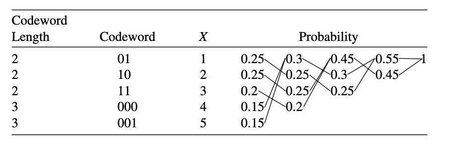
This code has average length 2.3 bits.

Optimality Of Huffman Coding

Theorem: Huffman coding is optimal; that is, if $C^{\ast }$ is a Huffman code and $C^{\prime }$ is any other uniquely decodable code, $L\left(C^{\ast }\right)\le L\left(C^{\prime }\right)$ .

In the following we'll proved the theorem for a binary alphabet, the proof can be extended for a D-ary alphabet as well.

It is important to remember that there are many optimal codes: inverting all the bits or exchanging two codewords of the same length will give another optimal code. The Huffman procedure constructs one such optimal code.

To prove the optimality of Huffman codes, we first prove some properties of a particular optimal code.

Without loss of generality, we will assume that the probability masses are ordered, so that $p_1\ge p_2\ge \cdots \ge p_m$. Recall that a code is optimal if $\sum p_i{l}_i$ is minimal.

Lemma

For any distribution, there exists an optimal instantaneous code (with minimum expected length) that satisfies the following properties:

1. The lengths are ordered inversely with the probabilities (i.e., if $p_j>$ $p_k$, then $l_j\le l_k$ ).
2. The two longest codewords have the same length.
3. Two of the longest codewords differ only in the last bit and correspond to the two least likely symbols.

Proof: The proof amounts to swapping, trimming, and rearranging, as shown in Figure 5.3. Consider an optimal code $C_m$ : - If $p_j>p_k$, then $l_j\le l_k$. Here we swap codewords. Consider $C_m^{\prime }$, with the codewords $j$ and $k$ of $C_m$ interchanged. Then

$$\begin{array}{rl}L\left(C_m^{\prime }\right)-L\left(C_m\right)& =\sum p_i{l}_i^{\prime }-\sum p_i{l}_i\\ & =p_j{l}_k+p_k{l}_j-p_j{l}_j-p_k{l}_k\\ & =(p_j-p_k)(l_k-l_j).\end{array}$$

But $p_j-p_k>0$, and since $C_m$ is optimal, $L\left(C_m^{\prime }\right)-L\left(C_m\right)\ge 0$. Hence, we must have $l_k\ge l_j$. Thus, $C_m$ itself satisfies property 1 . - The two longest codewords are of the same length. Here we trim the codewords. If the two longest codewords are not of the same length, one can delete the last bit of the longer one, preserving the prefix property and achieving lower expected codeword length. Hence, the two longest codewords must have the same length. By property 1 , the longest codewords must belong to the least probable source symbols. - The two longest codewords differ only in the last bit and correspond to the two least likely symbols. Not all optimal codes satisfy this property, but by rearranging, we can find an optimal code that does. If there is a maximal-length codeword without a sibling, we can delete the last bit of the codeword and still satisfy the prefix property. This reduces the average codeword length and contradicts the optimality of the code. Hence, every maximal-length codeword in any optimal code has a sibling. Now we can exchange the longest codewords so that the two lowest-probability source symbols are associated with two siblings on the tree. This does not change the expected length, $\sum p_i{l}_i$. Thus, the codewords for the two lowest-probability source symbols have maximal length and agree in all but the last bit.

Summarizing, we have shown that if $p_1\ge p_2\ge \cdots \ge p_m$, there exists an optimal code with $l_1\le l_2\le \cdots \le l_{m-1}=l_m$, and codewords $C\left(x_{m-1}\right)$ and $C\left(x_m\right)$ that differ only in the last bit.

Proof

Thus, we have shown that there exists an optimal code satisfying the properties of the lemma. We call such codes canonical codes.

For any probability mass function for an alphabet of size $m$, $$\mathbf{p}=(p_1,p_2,\dots ,p_m)$$

with $p_1\ge p_2\ge \cdots \ge p_m$,

we define the Huffman reduction $${\mathbf{p}}^{\prime }=(p_1,p_2,\dots ,p_{m-2},p_{m-1}+p_m)$$ over an alphabet of size $m-1$.

• Let $C_{m-1}^{\ast }\left({\mathbf{p}}^{\prime }\right)$ be an canonical optimal code for ${\mathbf{p}}^{\prime }$.
  • We denote the length of each codeword: $l_1^{\prime },l_2^{\prime },\cdots ,l_{m-1}^{\prime }$.
  • The average length is $L^{\ast }({\mathbf{p}}^{\prime })$.
• Let $C_m^{\ast }(\mathbf{p})$ be the canonical optimal code for $\mathbf{p}$.
  • We denote the length of each codeword: $l_1^{\prime },l_2^{\prime },\cdots ,l_m^{\prime }$.
  • The average length is $L^{\ast }(\mathbf{p})$.

The proof of optimality will follow from two constructions:

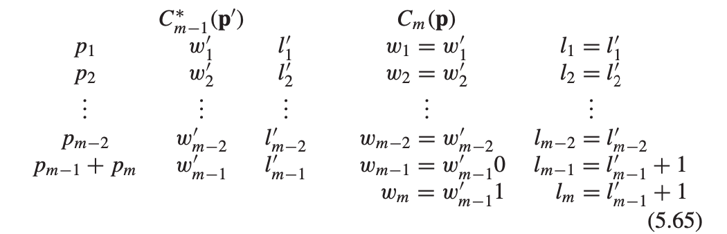
Step1

First, from the canonical code $C_{m-1}^{\ast }({\mathbf{p}}^{\prime })$ for ${\mathbf{p}}^{\prime }$, we construct a code $C_m(\mathbf{p})$ for $\mathbf{p}$: We find the codeword in that corresponds to weight $p_{m-1}+p_m$ and extend it by:

1. adding a 0 to form a codeword for symbol $m-1$
2. adding a 1 to form a codeword for symbol $m$.

The length of each codeword of $C_m(\mathbf{p})$ are: $$l_1,l_2,\cdots ,l_{m-2},l_{m-1},l_m=l_1^{\prime },l_2^{\prime },\cdots ,l_{m-2}^{\prime },l_{m-1}^{\prime }+1,l_{m-1}^{\prime }+1$$ The code construction is illustrated as follows:

Proof of optimality of Huffman coding

The average length of $C_m(\mathbf{p})$ is $$\begin{array}{rl}L(\mathbf{p})& =\sum _{i=1}^m{p}_i{l}_i\\ & =\sum _{i=1}^{m-2}{p}_i{l}_i+p_{m-1}\left(l_{m-1}\right)+p_m\left(l_m\right)\\ & =\sum _{i=1}^{m-2}{p}_i{l}_i^{\prime }+p_{m-1}(l_{m-1}^{\prime }+1)+p_m(l_{m-1}^{\prime }+1)\\ & =\sum _{i=1}^m{p}_i{l}_i^{\prime }+p_{m-1}+p_m\\ \text{(3)}& & =L^{\ast }\left({\mathbf{p}}^{\prime }\right)+p_{m-1}+p_m.\end{array}$$

Step2

Similarly, from the canonical code $C_m^{\ast }(\mathbf{p})$ for $\mathbf{p}$, we construct a code $C_{m-1}({\mathbf{p}}^{\prime })$ for ${\mathbf{p}}^{\prime }$: we use Huffman reduction to merge the codewords for the two lowest-probability symbols $m-1$ and $m$ with probabilities $p_{m-1}$ and $p_m$, which are siblings by the properties of the canonical code.

The average length of $C_{m-1}({\mathbf{p}}^{\prime })$ is $$\begin{array}{rl}L\left({\mathbf{p}}^{\prime }\right)& =\sum _{i=1}^{m-2}{p}_i{l}_i+p_{m-1}(l_{m-1}-1)+p_m(l_m-1)\\ & =\sum _{i=1}^m{p}_i{l}_i-p_{m-1}-p_m\\ \text{(4)}& & =L^{\ast }(\mathbf{p})-p_{m-1}-p_m.\end{array}$$

Step3

Adding $\text{(3)}$ and $\text{(4)}$ together, we obtain $$L\left({\mathbf{p}}^{\prime }\right)+L(\mathbf{p})=L^{\ast }\left({\mathbf{p}}^{\prime }\right)+L^{\ast }(\mathbf{p})$$ or $$(L\left({\mathbf{p}}^{\prime }\right)-L^{\ast }\left({\mathbf{p}}^{\prime }\right))+(L(\mathbf{p})-L^{\ast }(\mathbf{p}))=0.$$

We know that $L^{\ast }(\mathbf{p})$, $L^{\ast }({\mathbf{p}}^{\prime })$ are the optimal length for $\mathbf{p}$, ${\mathbf{p}}^{\prime }$. So we have:

1. $L(\mathbf{p})-L^{\ast }(\mathbf{p})\ge 0$.
2. $L\left({\mathbf{p}}^{\prime }\right)-L^{\ast }\left({\mathbf{p}}^{\prime }\right)\ge 0$.

If the sum of two nonnegative terms is 0, then both of them are 0, which implies that $L(\mathbf{p})=L^{\ast }(\mathbf{p})$ (i.e., the extension of the optimal code for ${\mathbf{p}}^{\prime }$ is optimal for $\mathbf{p}$) .

Conclustion

Consequently, if we start with an optimal code for ${\mathbf{p}}^{\prime }$ with $m-1$ symbols and construct a code for $m$ symbols by extending the codeword corresponding to $p_{m-1}+p_m$ , the new code is also optimal.

But how to start with an optimal code?

Well, we can start with a code for two elements, in which case the optimal code is obvious, we can by induction extend this result to prove the following theorem.