FIR Filters

Posted on 2023-11-23 Edited on 2024-09-17 In Electrical Engineering Views:

Sources:

James McClellan, Ronald Schafer & Mark Yoder. (2015). FIR Filters. DSP First (2nd ed., pp. 147-193). Pearson.

Discrete-Time Systems

Sequence: a discrete-time signal¹.
Discrete-time system or filter²: a function for transforming one sequence, called the input signal, into another sequence called the output signal.

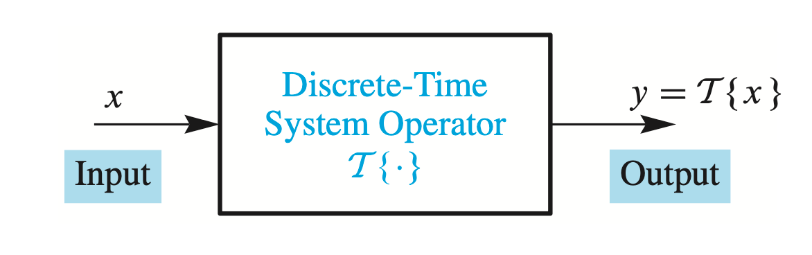
In general, we represent the operation of a discrete-time system by the notation \[ \begin{equation} \label{eq1.1} x[n] \stackrel{\mathcal{T}}{\longmapsto} y[n] \end{equation} \] Or \[ \begin{equation} \label{eq1.2} y[n] = \mathcal T (x[n]) \end{equation} \]

$x$: input sequence
$y$: output sequence
$\mathcal{T}$: the operator, aka computational process, mapping or function.

\[ y[n]=(x[n])^2 \]

The Running-Average Filter

A running average or moving average system: the output is the average of some consecutive values of the input. Such as \[ \begin{equation} \label{eq_difference equation} y[n] = \sum_{k=0}^{M} x[n-k] \end{equation} \] You can also define a running average as $y[n] = \sum_{k=0}^{M} x[n+k]$, $y[n] = \sum_{k=0}^{M} x[n-1+k]$ or whatever.
The equation like $\eqref{eq_difference equation}$ is called a difference equation. It is a complete description of the FIR system because we can use $\eqref{eq_difference equation}$ to compute the entire output signal for all index values $-\infty<n<\infty$.
A filter that uses only the present and past values of the input is called a causal filter. Thus $\eqref{eq_difference equation}$ is a causal running average.

Example

For a input sequence $x[n]$ with support set ${x[0], x[1], x[2]} = {2, 4, 6} $:

we define an output sequence $y[n]$:

Figure 5.2 b \[ \begin{equation} \label{eq_difference-equation-example} y[n]=\frac{x[n]+x[n+1]+x[n+2]}{3} \end{equation} \]

with \[ \begin{aligned} & y[0]=\frac{1}{3}(x[0]+x[1]+x[2]) \\ & y[1]=\frac{1}{3}(x[1]+x[2]+x[3]) \\ & \cdots \end{aligned} \]

$\eqref{eq_difference-equation-example}$ is the difference equation of this causal running average system.

The General FIR Filter

Definition

We define a $M^{\text{th}}$-order weighted running average/FIR filter of $M+1$ samples. \[ \begin{align} y[n] = \sum_{k=0}^M b_k x[n-k] \label{eq_FIR} , \end{align} \] which can be extended to $b_0 x[n]+b_1 x[n-1]+\cdots+b_M x[n-M]$.

FIR system: Finite Input Response system. Because the impulse response sequence $h[n]$ is finite(Illustrated later).
- $x[n], y[n]$ can be infinite since $n$ can be infinte: $- \infty < n < \infty$. But for FIR, the $h[n]$ must be finite.
The 3-point noncausal running average $\eqref{eq_difference equation-example}$ is the case where $M=2$ and $b_k=1 / 3$ in $\eqref{eq_FIR}$.
the coefficients $b_k$ are fixed numbers.
According to $\eqref{eq_FIR}$, an FIR filter is causal.
- Note that a noncausal system can be represented by altering $\eqref{eq_FIR}$ to include negative values of the summation index $k$.
Usually the $b_k$ coefficients are not all the same, and then we say that $\eqref{eq_FIR}$ is "weighted".
It follows from $\eqref{eq_FIR}$ that the computation of $y[n]$ involves the samples $x[\ell]$ for $\ell=n, n-1, n-2, \ldots, n-M$ (i.e., $x[n], x[n-1], x[n-2]$, etc):

A second defnition: \[ \begin{align} y[n] & = \sum_{\ell=n-M}^n b_{n-\ell} x[\ell] \label{eq_FIR2} , \end{align} \]

which can be extended to $b_M x[n-M]+b_{M-1} x[n-M+1]+\cdots+b_0 x[n]$.

Example

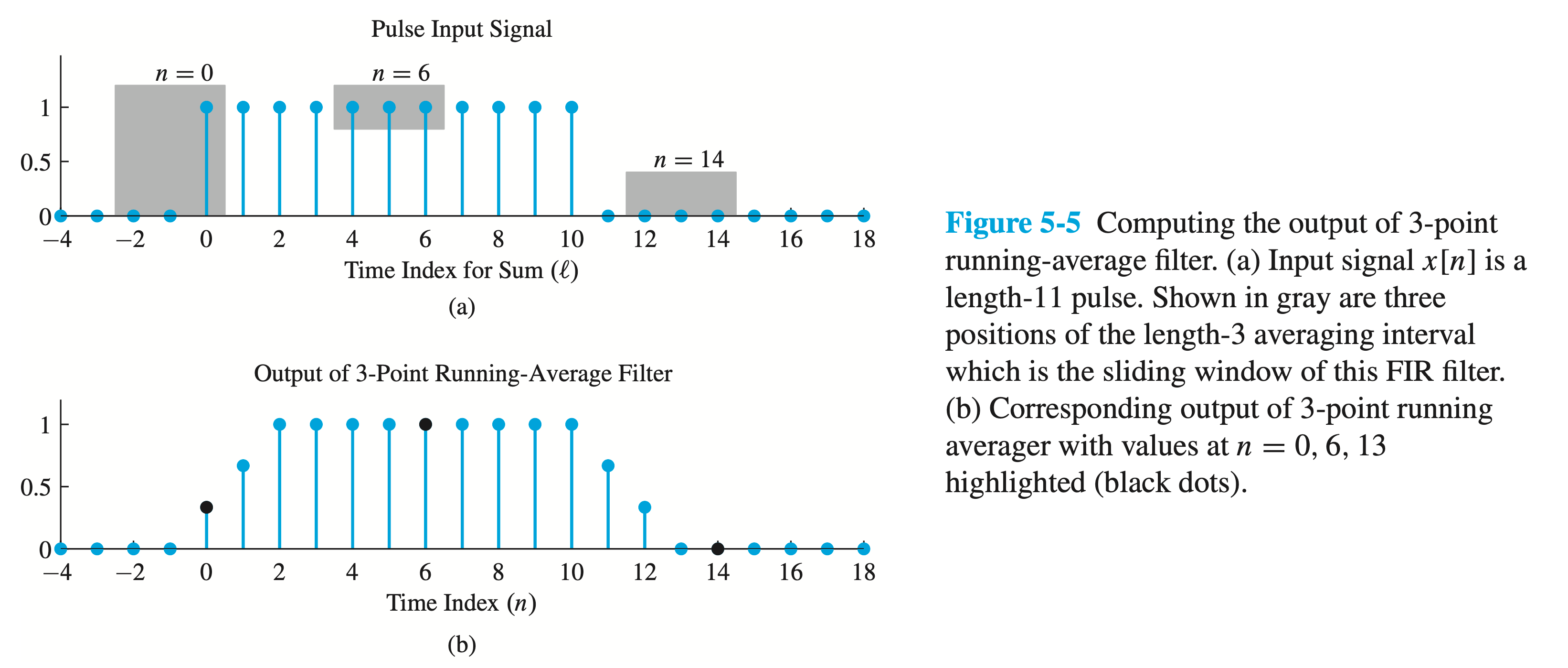
Figure 5.4 llustrates how the causal FIR filter uses $x[n]$ and the past $M$ samples to compute the output.

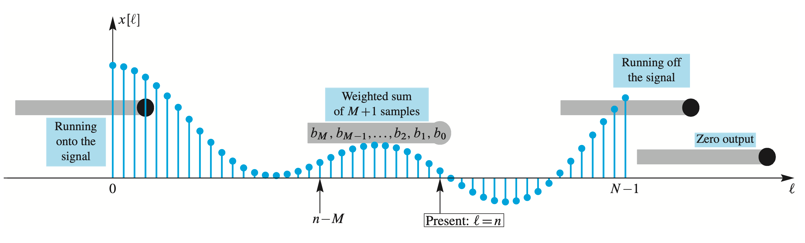
the weighted average is calculated over the (gray) sliding window of $M + 1$ samples.
When the input signal $x[l]$ has finite length ($N$ samples), the sliding window runs onto and off of the input data, so the resulting output signal also has finite length.

The Unit Impulse Response and Convolution

In this section, we introduce three new ideas: the unit impulse sequence, the unit impulse response, and the convolution sum.

We show that the impulse response provides a complete characterization of the FIR filter, because the convolution sum gives a formula for computing the output from the input when the unit impulse response is known.

Unit Impulse Sequence

The unit impulse: \[ \delta[n]= \begin{cases}1 & n=0 \\ 0 & n \neq 0\end{cases} \]

This notation is also known as the Kronecker delta function.

Shifted Unit Impulse Sequence

Here is the tabular of $\delta[n]$ and $\delta[n-2]$

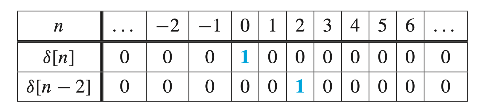
For a shifted unit impulse such as \[ \begin{equation} \label{eq_delay by 2} \delta[n-2] \end{equation} \]

The shifted impulse is a concept that is very useful in representing signals and systems. For example, we can show that the formula \[ x[n]=2 \delta[n]+4 \delta[n-1]+6 \delta[n-2]+4 \delta[n-3]+2 \delta[n-4] \] is equivalent to defining $x[n]$ by tabulating its five nonzero values:

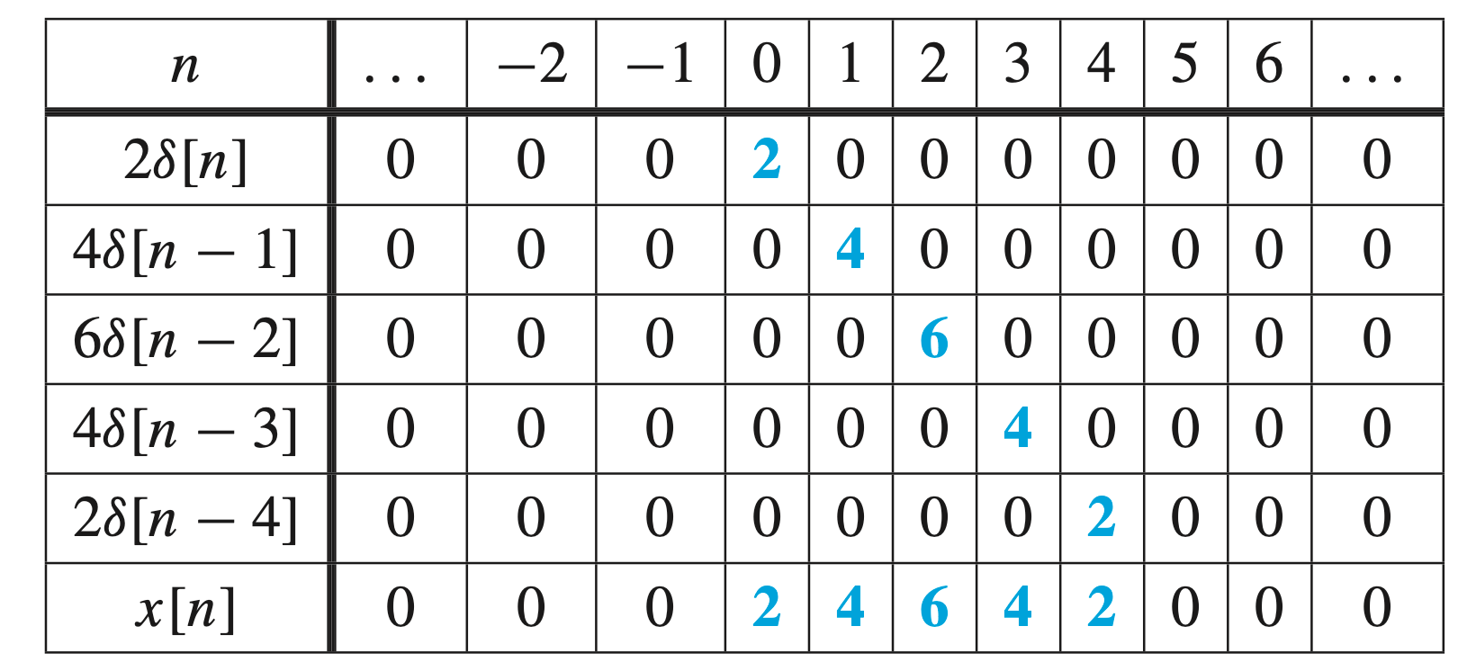
It turns out that any sequence³ can be represented by a sum of scaled shifted impulses . The equation \[ \begin{aligned} x[n] & =\sum_k x[k] \delta[n-k] \\ & =\cdots+x[-1] \delta[n+1]+x[0] \delta[n]+x[1] \delta[n-1]+x[2] \delta[n-2]+\cdots \end{aligned} \] is true if $k$ ranges over all the nonzero values of the sequence $x[n]$.

Unit Impulse Response Sequence

The output from a filter is often called the response to the input.
When the input is the unit impulse, $\delta[n]$, the output is called the unit impulse response (Or impulse response, with unit being understood).
Notation of unit impulse response: ${h}[n]$.
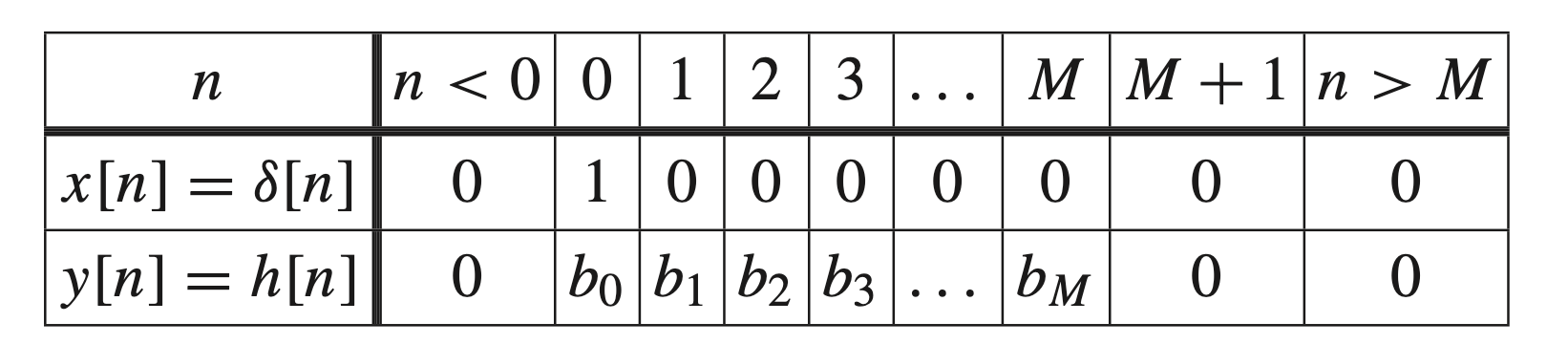
When the input to the FIR filter $\eqref{eq_FIR}$ is a unit impulse sequence, $x[n]=\delta[n]$, the output is the (unit) impulse response $h[n]$. Substituting $x[n]=\delta[n]$ in $\eqref{eq_FIR}$ gives the output $y[n]=h[n]$: \[ h[n]=\sum_{k=0}^M b_k \delta[n-k]= \begin{cases}b_n & n=0,1,2, \ldots, M \\ 0 & \text { otherwise }\end{cases} \]

Note that because each $\delta[n-k]$ is nonzero only when $n-k=0$, or $n=k$, the impulse response is:
In other words, the impulse response ${h}[n]$ of the FIR filter is identical to the sequence of difference equation coefficients. So the FIR filter is completely defined by the impulse response.
- In following chapter, we'll show that this characterization is also true for the much broader class of linear time-invariant (LTI) systems.
Since $h[n]=0$ for $n<0$ and for $n>M$, the "length"⁴ of the impulse response sequence $h[n]$ is finite. This is why the system $\eqref{eq_FIR}$ is called a FIR system.

The Unit-Delay System

One important system is the operator that performs a delay or shift by an amount $n_0$ \[ y[n]=x\left[n-n_0\right] \]

When $n_0=1$, the system is called a unit delay.

The delay system is actually the simplest of FIR filters. \[ \begin{aligned} y[n] & =b_0 x[n]+b_1 x[n-1]+b_2 x[n-2]+ \cdots + b_{n_0} x[n-n_0] \\ & =(0) x[n]+(0) x[n-1]+(0) x[n-2] + \cdots + (1) x[n-n_0] \\ & =x[n-n_0] \end{aligned} \]
The impulse response of the delay system is obtained by substituting $\delta[n]$ for $x[n]$.
$\eqref{eq_delay by 2}$ is a delay-by-2 system $y[n] = x[n-2]$ with coefficients $\left\{b_k\right\}=$ $\{0,0,1\}$, its impulse response is: \[ h[n]=\delta\left[n-n_0\right]=\delta[n-2]= \begin{cases}1 & n=2 \\ 0 & n \neq 2\end{cases} \]

FIR Filters and Convolution

Since the filter coefficients in $\eqref{eq_FIR}$ are identical to the impulse response value $h[n]$. We can express a FIR filter in terms of the input and the impulse response. This is called convolution sum: \[ \begin{equation} \label{eq_convolution-sum} y[n]=\sum_{k=0}^M h[k] x[n-k] \end{equation} \] Here we replace $b_k$ in $\eqref{eq_FIR}$ with $h[k]$.

The terminology convolution emphasizes that it's an operation between two sequences.
We use a star $(*)$ to represent the operation of evaluating (5.13) for $-\infty<$ $n<\infty$ by writing \[ \begin{equation} \label{eq_convolution sum star} y[n]=h[n] * x[n] \end{equation} \] which is read as "the output sequence $y[n]$ is obtained by convolving the impulse response $h[n]$ with the input sequence $x[n]$."

Later, in Section 5-7, we will prove that convolution is the fundamental input-output algorithm for a large class of very useful filters that includes FIR filters as a special case. We will show that a general form of convolution that also applies to infinite-length signals is \[ \begin{align} y[n] & = h[n] * x[n] \nonumber \\ & = \sum_{k=-\infty}^{\infty} h[k] x[n-k] \label{eq_convolution sum inf} . \end{align} \]

This convolution sum $\eqref{eq_convolution sum inf}$ has infinite limits to accomodate impulse responses of infinite length, but reduces to $\eqref{eq_convolution-sum}$ when $h[n]=0$ for $n<0$ and $n>M$.

The Length of a Convolution

If $x[n]$ is nonzero only in the interval $0 \leq n \leq L_x-1$, then for a causal FIR filter having an impulse response of length $L_h=M+1$ samples (because the impulse response is the sequence: h[0], h[1], ..., h[M]), the corresponding output $y[n]$, which is the convolution of $h[n]$ with $x[n]$, can be nonzero only when $n \geq 0$ and $n-M \leq L_x-1$, or equivalently, the support set of $y[n]$ is the interval $0 \leq n \leq L_x+M-1$. Thus the length of $y[n]$ is \[ \begin{equation} \label{eq_convolution length} L_y=L_x+L_h-1 \end{equation} \]

通俗地说, $y[n]$长度 = $x[n]$长度 + $h[n]$长度 - 1.

以下面example为例, $x[n]$的长度是11($L_x = 11$), 最后一个非0值位于下标10($L_x-1$), 但由于$M=3$, 因此以$x[10]$为起始点的$M$个值 $x[10], x[11], x[12]$的running average 还是非零: \[ y[12] = x[12] * h[12] \ne 0 , \] convolution一直持续到下标12($L_x -1 +M $).

而convolution是从下标0开始的($\frac{Px[-2]+x[-1]+x[-1]}{3}$), 因此convolution $y[n]$从下标0一直持续到下标12($L_x -1 +M$). 其长度为$L_x + M = L_y=L_x+L_h-1$.

When the signals start at $n=0$, it is possible to use the synthetic multiplication table to prove that the formula $\eqref{eq_convolution length}$ is true. Since the length of $x[n]$ is $L_x$, the last nonzero signal value is $x\left[L_x-1\right]$. Likewise, for $h[n]$ where $h\left[L_h-1\right]$ is the last nonzero value. In the figure, the row for $h[0] x[n]$ starts at $n=0$ and ends at $n=L_x-1$, while the row for $h\left[L_h-1\right] x\left[n-\left(L_h-1\right)\right]$ ends at $n=\left(L_x-1\right)+\left(L_h-1\right)$. After summing down the columns, we see that the convolution result $y[n]$ starts at $n=0$ and ends at $n=L_h+L_x-2$, so the length of $y[n]$ is $L_x+L_h-1$. Problem P-5.6 considers the general case where the signal $x[n]$ begins at sample $N_1$ and ends at sample $N_2$.

Example

Given impulse response \[ h[n]=\frac{1}{3} \delta[n]+\frac{1}{3} \delta[n-1]+\frac{1}{3} \delta[n-2] \] and input $x[n] = \begin{cases} 1 & n=0,1,2, \ldots, 10 \\ 0 & \text { otherwise }\end{cases}$.

The output $y[n] = h[n] * x[n]$ has length $L_y=11+3-1=13$.

Filtering the Unit-Step Signal

In previous sections, we have described the FIR filtering of finite-length signals.

But the input signal can also have infinite duration.

An example is the unit-step signal which is zero for $n<0$ and "turns on" at $n=0$ \[ u[n]= \begin{cases}0 & n<0 \\ 1 & n \geq 0\end{cases} \]

The symbol $u[n]$ is reserved for the unit step.

So when we want the input signal to be the unit step we write $x[n]=u[n]$, and the output of an $M^{\text {th }}$-order FIR filter would be \[ y[n]=\sum_{\ell=n-M}^n b_{n-\ell} u[\ell] \] if we use the form in $\eqref{eq_FIR}$. Since the FIR filter is causal and the unit step starts at $n=0$, the output is zero for $n<0$. Determining the output for $n \geq 0$ can be done by writing out terms

Property of Convolution

convolution is:

commutative: $y[n] = h[n] * x[n] = x[n] * h[n]$

//Proof: TODO

See↩︎
Strictly speaking, a filter is a system that is designed to remove some component or modify some characteristic of a signal, but often the two terms are used interchangeably.↩︎
Remember that a sequence is a discrete-time signal.↩︎
这里所谓"length"指的是support set的长度. n可以是无限的, 因此$x[n], y[n], h[n]$也可以是无限的. 但是它们的suport set未必无限. 特别是$h[n]$的长度已经被$\eqref{eq_convolution-sum}$固定为$M+1$.↩︎