Frequency Response of FIR Filters

Posted on 2023-11-22 Edited on 2024-09-17 In Electrical Engineering Views:

Sources:

Jiames McClellan, Ronald Schafer & Mark Yoder. (2015). Sinusoids. DSP First (2nd ed., pp. 9-40). Pearson.

Sinusoidal Response of FIR Systems

Given an input that is a complex exponential signal \[ \begin{equation} \label{eq_complex exponential signal} x[n]=A e^{j \varphi} e^{j \hat\omega n} \quad-\infty<n<\infty . \end{equation} \]

Recall that a discrete-time signal could have been obtained by sampling a continuous-time signal.

Given $x(t)=A e^{j \varphi} e^{j \omega t}$. Then we can get $x[n]=x\left(n T_s\right)$. $\omega$ and $\hat{\omega}$ are related by $\hat{\omega}=\omega T_s$, where $T_s$ is the sampling period.

Consider an FIR system \[ \begin{equation} \label{FIR} y[n]=\sum_{k=0}^M b_k x[n-k] , \end{equation} \] the corresponding output is \[ \begin{align} y[n] & =\sum_{k=0}^M b_k A e^{j \varphi} e^{j \hat{\omega}(n-k)} \nonumber \\ & =\left(\sum_{k=0}^M b_k e^{-j \hat{\omega} k}\right) A e^{j \varphi} e^{j \hat{\omega} n} \nonumber \\ & =\mathcal{H}(\hat{\omega}) A e^{j \varphi} e^{j \hat{\omega} n} \label{eq_output} \end{align} \] with $-\infty<n<\infty$,

where \[ \begin{equation} \label{eq_frequency_response} \mathcal{H}(\hat{\omega})=\sum_{k=0}^M b_k e^{-j \hat{\omega} k} \end{equation} \]

To emphasize the ubiquity of $e^{j \hat{\omega}}$, in $\eqref{eq_frequency_response}$ we usually use the notation $H\left(e^{j \hat{\omega}}\right)$ instead of $\mathcal{H}(\hat{\omega})$.

$H\left(e^{j \hat{\omega}}\right)$ : frequency response, the frequency response function of the LTI system.
$H\left(e^{j \hat{\omega}}\right)$ is complex valued. So it can be expressed either as \[ \begin{equation} \label{eq_Cartesian_form} \left|H\left(e^{j \hat{\omega}}\right)\right| e^{j \angle H\left(e^{j \hat{\omega}}\right)} \end{equation} \] or as \[ \begin{align} \Re\left\{H\left(e^{j \hat{\omega}}\right)\right\}+j \Im\left\{H\left(e^{j \hat{\omega}}\right)\right\} \label{eq_Polar-form} . \end{align} \] where:
- $\left|H\left(e^{j \hat{\omega}}\right)\right|$: the magnitute of $H\left(e^{j \hat{\omega}}\right)$.
- $\angle H\left(e^{j \hat{\omega}}\right)$: the angle or phase of $H\left(e^{j \hat{\omega}}\right)$.
- For instance, if $H\left(e^{j \hat{\omega}}\right) = 3 e^{-j \pi / 3}$, then the magnitude is $\left|H\left(e^{j \hat{\omega}}\right)\right|$ = 3, the angle is $\angle H\left(e^{j \hat{\omega}}\right) = - \pi / 3$.
Ideas:
1. $\eqref{eq_output}$ shows that when the input is a discrete-time complex exponential signal, the output of an LTI FIR filter is also a discretetime complex exponential signal with the same frequency $\hat{\omega}$, but with different magnitude and phase.
2. The mathematical statement $y[n]=H\left(e^{j \hat{\omega}}\right) x[n]$ is true iff for input signals of precisely the form $\eqref{eq_complex exponential signal}$. Otherwise this statement is meaningles.
Using the polar form $\eqref{eq_Polar-form}$ in $\eqref{eq_output}$ gives the result \[ \begin{aligned} y[n] & = H\left(e^{j \hat{\omega}}\right) A e^{j \varphi} e^{j \hat{\omega} n} \\ & = \ \left(\left|H\left(e^{j \hat{\omega}}\right)\right| e^{j \angle H e^{j \hat{\omega}}}\right) A e^{j \varphi} e^{j \hat{\omega} n} \\ & = \left(\left|H\left(e^{j \hat{\omega}}\right)\right| A\right) e^{j \angle H\left(e^{j \hat{\omega}}+\varphi\right)} e^{j \hat{\omega} n} \end{aligned} \]

As a result, we have: \[ \color{red} y[n] = \left(\left|H\left(e^{j \hat{\omega}}\right)\right| A\right) e^{j \angle H\left(e^{j \hat{\omega}}+\varphi\right)} e^{j \hat{\omega} n} \label{eq1.1.1} \]
- The magnitude of $H\left(e^{j \hat{\omega}}\right)$ multiplies the signal amplitude $(A)$ which changes the size of the signal. Thus, $\left|H\left(e^{j \hat{\omega}}\right)\right|$ is usually referred to as the gain of the system.¹
- The angle $\angle H\left(e^{j \hat{\omega}}\right)$ simply adds to the phase $(\varphi)$ of the input, thereby producing additional phase shift in the complex exponential signal.
For an FIR filter:

frequency response $H\left(e^{j \hat{\omega}}\right)$ <==> impulse response $h[k]$ <==> the sequence of filter coefficients $b_k$ .

That is, \[ \begin{align} & H\left(e^{j \hat{\omega}}\right) \nonumber \\ = \quad & \sum_{k=0}^M b_k e^{-j \hat{\omega} k} \nonumber \\ = \quad & \sum_{k=0}^M h[k] e^{-j \hat{\omega} k} \label{eq1.1.2} \end{align} \]
Time Domain <--> Frequency Domain

\[ \begin{aligned} & \text { Time Domain } \longleftrightarrow \text { Frequency Domain } \\ & h[n]=\sum_{k=0}^M h[k] \delta[n-k] \longleftrightarrow H\left(e^{j \hat{\omega}}\right)=\sum_{k=0}^M h[k] e^{-j \hat{\omega} k} \\ & \end{aligned} \]

Example: Formula for the Frequency Response

Consider an LTI system for which the difference equation coefficients are $\left\{b_k\right\}=\{1,2,1\}$. Substituting into $\eqref{eq_frequency_response}$ gives \[ H\left(e^{j \hat{\omega}}\right)=1+2 e^{-j \hat{\omega}}+e^{-j \hat{\omega} 2} \]

To obtain formulas for the magnitude and phase of the frequency response of this FIR filter, we can manipulate the equation as follows: \[ \begin{align} H\left(e^{j \hat{\omega}}\right) & =1+2 e^{-j \hat{\omega}}+e^{-j \hat{\omega} 2} \nonumber \\ & =e^{-j \hat{\omega}}\left(e^{j \hat{\omega}}+2+e^{-j \hat{\omega}}\right) \nonumber \\ & =e^{-j \hat{\omega}}(2+2 \cos \hat{\omega}) \label{eq1.2.1} \end{align} \]

$\eqref{eq1.2.1}$ is due to the inverse Eula formulas.

Since $(2+2 \cos \hat{\omega}) \geq 0$ for frequencies $-\pi<\hat{\omega} \leq \pi$, recall $\eqref{eq_Cartesian_form}$, the magnitude is $\left|H\left(e^{j \hat{\omega}}\right)\right|=$ $(2+2 \cos \hat{\omega})$ and the phase is $\angle H\left(e^{j \hat{\omega}}\right)=-\hat{\omega}$.

Example: Complex Exponential Input

Consider the complex input $x[n]=2 e^{j \pi / 4} e^{j(\pi / 3) n}$ whose frequency is $\hat{\omega}=\pi / 3$ and the system in the last Example.

To get the output, we can evaluate the frequency response at the input frequency using the method defined in $\eqref{eq1.1.1}$.

The evaluation gives: $\left|H\left(e^{j \pi / 3}\right)\right|=2+2 \cos (\pi / 3)$=3 and $\angle H\left(e^{j \pi / 3}\right)=-\pi / 3$.

Therefore, the output of the system for the given input is \[ \begin{aligned} y[n] & =3 e^{-j \pi / 3} \cdot 2 e^{j \pi / 4} e^{j \pi n / 3} \\ & =(3 \cdot 2) \cdot e^{(j \pi / 4-j \pi / 3)} e^{j \pi n / 3} \\ & =6 e^{-j \pi / 12} e^{j \pi n / 3}=6 e^{j \pi / 4} e^{j \pi(n-1) / 3} \end{aligned} \]

Thus, for this system and the given input $x[n]$, the output is equal to the input multiplied by 3 , and the phase shift of $-\pi / 3$ corresponds to a delay of one sample.

Example: $h[n] \longleftrightarrow H\left(e^{j \hat{\omega}}\right)$

Consider the FIR filter defined by the impulse response \[ h[n]=-\delta[n]+3 \delta[n-1]-\delta[n-2] \]

The values of $h[n]$ are the filter coefficients $\left\{b_k\right\}=\{-1,3,-1\}$, so the difference equation corresponding to this impulse response is \[ y[n]=-x[n]+3 x[n-1]-x[n-2] \]

Thus, the frequency response of this system is \[ H\left(e^{j \hat{\omega}}\right)=-1+3 e^{-j \hat{\omega}}-e^{-j 2 \hat{\omega}} \]

Example: Difference Equation from $H\left(e^{j \hat{\omega}}\right)$

Often the frequency response is given by an equation containing sines or cosines, for example, \[ H\left(e^{j \hat{\omega}}\right)=e^{-j \hat{\omega}}(3-2 \cos \hat{\omega}) \]

To obtain the FIR difference equation, it is necessary to write $H\left(e^{j \hat{\omega}}\right)$ using powers of $e^{-j \hat{\omega}}$. In this example, we can use the inverse Euler formula $\cos \hat{\omega}=\frac{1}{2}\left(e^{j \hat{\omega}}+e^{-j \hat{\omega}}\right)$, and then obtain \[ \begin{aligned} H\left(e^{j \hat{\omega}}\right) & =e^{-j \hat{\omega}}\left[3-2\left(\frac{e^{j \hat{\omega}}+e^{-j \hat{\omega}}}{2}\right)\right] \\ & =-1+3 e^{-j \hat{\omega}}-e^{-j \hat{\omega} 2} \end{aligned} \]

Now, it should be easy to see that $H\left(e^{j \hat{\omega}}\right)$ corresponds to the following FIR difference equation: \[ y[n]=-x[n]+3 x[n-1]-x[n-2] \]

The impulse response, likewise, is easy to determine directly from $H\left(e^{j \hat{\omega}}\right)$, when expressed in terms of powers of $e^{-j \hat{\omega}}$.

Superposition and the Frequency Response

We can easily apply the principle of superposition in frequency domain:

If the input signal consists of the sum of many complex exponential signals, the frequency response can be applied to find the output due to each component separately, and the results added to determine the total output.

Cosine in, Cosine out

Theorem: For every cosine input signal, the system still outputs cosine signals.

That is, for input like \[ x[n]=\sum_{k=0}^M b_k x[n-k] =\sum_{k=0}^M b_k \cos(w_k n + \varphi_k) , \] the output is \[ y[n]=\sum_{k=0}^M |H\left(e^{j \hat{\omega}_k}\right)| b_k \cos(w_k n + \varphi_k + \angle H\left(e^{j \hat{\omega}_k}\right)). \]

As an example, suppose that the input to an LTI system is a cosine wave with a specific normalized frequency $\hat{\omega}_1$ plus a DC level, \[ \begin{equation} \label{eq2.1.1} x[n]=A_0+A_1 \cos \left(\hat{\omega}_1 n+\varphi_1\right) \end{equation} \]

If we represent the signal in terms of complex exponentials, note that $A_0 = A_0 e^0$, the signal is composed of three complex exponential signals, with frequencies $\hat{\omega}=0, \hat{\omega}_1$, and $-\hat{\omega}_1$, so \[ x[n]=A_0 e^{j 0 n}+\frac{A_1}{2} e^{j \varphi_1} e^{j \hat{\omega}_1 n}+\frac{A_1}{2} e^{-j \varphi_1} e^{-j \hat{\omega}_1 n} \]

By superposition, we cam determine the output just multiply each component by $H\left(e^{j \hat{\omega}}\right)$ evaluated at the corresponding frequency: \[ y[n]=H\left(e^{j 0}\right) A_0 e^{j 0 n}+H\left(e^{j \hat{\omega}_1}\right) \frac{A_1}{2} e^{j \varphi_1} e^{j \hat{\omega}_1 n}+H\left(e^{-j \hat{\omega}_1}\right) \frac{A_1}{2} e^{-j \varphi_1} e^{-j \hat{\omega}_1 n} \]

Then we use $\eqref{eq_Cartesian_form}$ to express $H\left(e^{j \hat{\omega}_1}\right)$, $y[n]$ can finally be expressed as

$$ \[\begin{aligned} y[n] & = H\left(e^{j 0}\right) A_0 e^{j 0 n}+H\left(e^{j \hat{\omega}_1}\right) \frac{A_1}{2} e^{j \varphi_1} e^{j \hat{\omega}_1 n}+H^*\left(e^{j \hat{\omega}_1}\right) \frac{A_1}{2} e^{-j \varphi_1} e^{-j \hat{\omega}_1 n} \\ & = H\left(e^{j 0}\right) A_0+\left|H\left(e^{j \hat{\omega}_1}\right)\right| e^{j \angle H\left(e^{j \hat{\omega}_1}\right)} \frac{A_1}{2} e^{j \varphi_1} e^{j \hat{\omega}_1 n} + \left|H\left(e^{j \hat{\omega}_1}\right)\right| e^{-j \angle H\left(e^{j \hat{\omega}_1}\right)} \frac{A_1}{2} e^{-j \varphi_1} e^{-j \hat{\omega}_1 n} \\ & = H\left(e^{j 0}\right) A_0+\left|H\left(e^{j \hat{\omega}_1}\right)\right| \frac{A_1}{2} e^{j\left(\hat{\omega}_1 n+\varphi_1+\angle H\left(e^{j \hat{\omega}_1}\right)\right)} +\left|H\left(e^{j \hat{\omega}_1}\right)\right| \frac{A_1}{2} e^{-j\left(\hat{\omega}_1 n+\varphi_1+\angle H\left(e^{j \hat{\omega}_1}\right)\right)} \\ & = H\left(e^{j 0}\right) A_0+\left|H\left(e^{j \hat{\omega}_1}\right)\right| A_1 \cos \left(\hat{\omega}_1 n+\varphi_1+\angle H\left(e^{j \hat{\omega}_1}\right)\right) \end{aligned}\]

$$ The deduction from the first line to the second line is because we assume $H\left(e^{j \hat{\omega}_1}\right)$ has conjugate symmetry here. This assumption is always true when the filter coefficients are real.

Example: Cosine Input

Consider the complex input \[ x[n]=3 \cos \left(\frac{\pi}{3} n-\frac{\pi}{2}\right) \] and the system in the previous Example.

To get the output, we first know from the previous example that \[ H\left(e^{j \hat{\omega}}\right)=(2+2 \cos \hat{\omega}) e^{-j \hat{\omega}} \]

Then we evaluate $H\left(e^{j \hat{\omega}}\right)$ at the frequency $\hat{\omega}=\pi / 3$ : \[ \begin{aligned} H\left(e^{j \pi / 3}\right) & =e^{-j \pi / 3}(2+2 \cos (\pi / 3)) \\ & =e^{-j \pi / 3}\left(2+2\left(\frac{1}{2}\right)\right)=3 e^{-j \pi / 3} \end{aligned} \]

Therefore, the magnitude is $\left|H\left(e^{j \pi / 3}\right)\right|=3$ and the phase is $\angle H\left(e^{j \pi / 3}\right)=-\pi / 3$.

From $\eqref{eq2.1.3}$, when conjugate symmetry holds, the output is \[ \begin{aligned} y[n] & =(3)(3) \cos \left(\frac{\pi}{3} n-\frac{\pi}{3}-\frac{\pi}{2}\right) \\ & =9 \cos \left(\frac{\pi}{3}(n-1)-\frac{\pi}{2}\right) \end{aligned} \]

That is, the magnitude of the frequency response multiplies the amplitude of the cosine signal, and the phase angle of the frequency response adds to the phase of the cosine signal.

For Real Signal

For real signals($x[n]\in \mathbb R$), we can still apply frequency reponses by converting it to complex exponential signals: \[ \begin{aligned} x[n] & =X_0+\sum_{k=1}^N\left(\frac{X_k}{2} e^{j \hat{\omega}_k n}+\frac{X_k^*}{2} e^{-j \hat{\omega}_k n}\right) \\ & =X_0+\sum_{k=1}^N\left|X_k\right| \cos \left(\hat{\omega}_k n+\angle X_k\right) \end{aligned} \]

then the corresponding output $y[n]$ is: \[ \begin{aligned} y[n] & =H\left(e^{j 0}\right) X_0+\sum_{k=1}^N\left(H\left(e^{j \hat{\omega}_k}\right) \frac{X_k}{2} e^{j \hat{\omega}_k n}+H\left(e^{-j \hat{\omega}_k}\right) \frac{X_k^*}{2} e^{-j \hat{\omega}_k n}\right) \\ & =H\left(e^{j 0}\right) X_0+\sum_{k=1}^N\left|H\left(e^{j \hat{\omega}_k}\right)\right|\left|X_k\right| \cos \left(\hat{\omega}_k n+\angle X_k+\angle H\left(e^{j \hat{\omega}_k}\right)\right) \end{aligned} \]

Example: Three Sinusoidal Inputs

Consider the complex input: \[ x[n]=4+3 \cos \left(\frac{\pi}{3} n-\frac{\pi}{2}\right)+3 \cos \left(\frac{7 \pi}{8} n\right) \]

and the system in the previous Example. Find the output.

We evaluate $H\left(e^{j \hat{\omega}}\right)$ at frequencies $0, \pi / 3$, and $7 \pi / 8$, giving \[ \begin{aligned} H\left(e^{j 0}\right) & =4 \\ H\left(e^{j \pi / 3}\right) & =3 e^{-j \pi / 3} \\ H\left(e^{j 7 \pi / 8}\right) & =0.1522 e^{-j 7 \pi / 8} \end{aligned} \]

Therefore, the output is \[ \begin{aligned} y[n] & =4 \cdot 4+3 \cdot 3 \cos \left(\frac{\pi}{3} n-\frac{\pi}{3}-\frac{\pi}{2}\right)+0.1522 \cdot 3 \cos \left(\frac{7 \pi}{8} n-\frac{7 \pi}{8}\right) \\ & =16+9 \cos \left(\frac{\pi}{3}(n-1)-\frac{\pi}{2}\right)+0.4567 \cos \left(\frac{7 \pi}{8}(n-1)\right) \end{aligned} \]

Notice that the component at frequency $\hat{\omega}=7 \pi / 8$ is multiplied by 0.1522 . Because the frequency-response magnitude (gain) is so small at frequency $\hat{\omega}=7 \pi / 8$, the component at this frequency is essentially filtered out of the input signal.

Steady-State and Transient Response

In Section 6-1, we showed that if the input is \[ x[n]=X e^{j \hat{\omega} n} \quad-\infty<n<\infty \] where $X=A e^{j \varphi}$, then the corresponding output of an LTI FIR system is \[ y[n]=H\left(e^{j \hat{\omega}}\right) X e^{j \hat{\omega} n} \quad-\infty<n<\infty \] where \[ H\left(e^{j \hat{\omega}}\right)=\sum_{k=0}^M b_k e^{-j \hat{\omega} k} \]

In (6.9), the condition that $x[n]$ be a complex exponential signal existing over $-\infty<n<\infty$ is important. Without this condition, we cannot obtain the simple result of (6.10).

However, this condition appears to be somewhat impractical. In any practical implementation, we surely would not have actual input signals that exist back to $-\infty$ !

Fortunately, we can relax the condition that the complex exponential input be defined over the doubly infinite interval and still take advantage of the convenience of (6.10). To see this, consider the following "suddenly applied" complex exponential signal that starts at $n=0$ and is nonzero only for $0 \leq n$ : \[ x[n]=X e^{j \hat{\omega} n} u[n]= \begin{cases}X e^{j \hat{\omega} n} & 0 \leq n \\ 0 & n<0\end{cases} \]

Note that multiplication by the unit-step signal is a convenient way to impose the suddenly applied condition. The output of an LTI FIR system for this input is obtained by using the definition of $x[n]$ in (6.12) in the FIR difference equation: \[ y[n]=\sum_{k=0}^M b_k \underbrace{X e^{j \hat{\omega}(n-k)} u[n-k]}_{x[n-k]} \] By considering different values of $n$ and the fact that $u[n-k]=0$ for $k>n$, it follows that the sum in (6.13) can be expressed as three cases \[ y[n]= \begin{cases}0 & n<0 \\ \left(\sum_{k=0}^n b_k e^{-j \hat{\omega} k}\right) X e^{j \hat{\omega} n} & 0 \leq n<M \\ \left(\sum_{k=0}^M b_k e^{-j \hat{\omega} k}\right) X e^{j \omega \hat{n}} & M \leq n\end{cases} \]

That is, when the complex exponential signal is suddenly applied, the output can be considered to be defined over three distinct regions. In the first region, $n<0$, the input is zero, and therefore the corresponding output is zero, too. The second region is a transition region whose length is $M$ samples (i.e., the order of the FIR system). In this region, the complex multiplier of $e^{j \hat{\omega} n}$ depends upon $n$. This region is often called the transient part of the output. In the third region, $M \leq n$, the output is identical to the output that would be obtained if the input were defined over the doubly infinite interval, that is, \[ y[n]=H\left(e^{j \hat{\omega}}\right) X e^{j \omega \hat{n}} \quad M \leq n \]

This part of the output is generally called the steady-state part. While we have specified that the steady-state part exists for all $n \geq M$, it should be clear that (6.15) holds only as long as the input remains equal to $X e^{j \hat{\omega} n}$. If, at some time $n>M$, the input changes frequency or the amplitude becomes zero, another transient region occurs.

Example: Steady-State Output

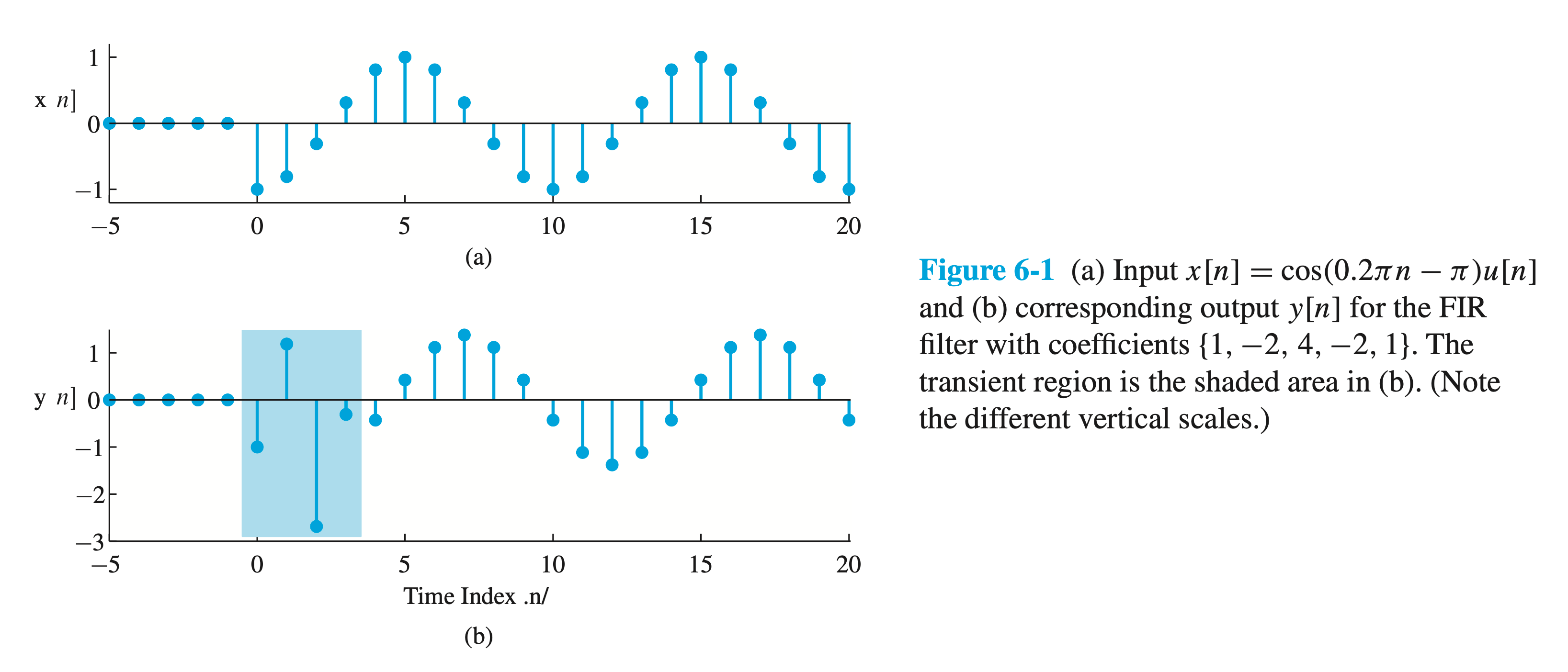
A simple example illustrates the above discussion. Consider the system of Exercise 6.1, whose filter coefficients are the sequence $\left\{b_k\right\}=\{1,-2,4,-2,1\}$. The frequency response of this system is \[ H\left(e^{j \hat{\omega}}\right)=[4-4 \cos (\hat{\omega})+2 \cos (2 \hat{\omega})] e^{-j 2 \hat{\omega}} \]

If the input is the suddenly applied cosine signal \[ x[n]=\cos (0.2 \pi n-\pi) u[n] \] we can represent it as the sum of two suddenly applied complex exponential signals. Therefore, the frequency response can be used as discussed in Section 6-2 to determine the corresponding steady-state output. Since $H\left(e^{j \hat{\omega}}\right)$ at $\hat{\omega}=0.2 \pi$ is \[ H\left(e^{j \hat{\omega}}\right)=[4-4 \cos (0.2 \pi)+2 \cos (0.4 \pi)] e^{-j 2(0.2 \pi)}=1.382 e^{-j(0.2 \pi) 2} \] and $M=4$, the steady-state output is \[ y[n]=1.382 \cos (0.2 \pi(n-2)-\pi) \quad 4 \leq n \]

The frequency response has allowed us to find a simple expression for the output everywhere in the steady-state region. If we desire the values of the output in the transient region, we could compute them using the difference equation for the system.

The input and output signals for this example are shown in Fig. 6-1. Since $M=4$ for this system, the transient region is $0 \leq n \leq 3$ (indicated by the shaded region), and the steady-state region is $n \geq 4$. Also note that, as predicted by the steady-state analysis above, the signal in the steady-state region is simply a scaled (by 1.382) and shifted (by two samples) version of the input. 6-4 Properties of the Frequency Response

Properties of the Frequency Response

The frequency response $H\left(e^{j \hat{\omega}}\right)$ is a complex-valued function of the normalized frequency variable $\hat{\omega}$.

This function has interesting properties that often can be used to simplify analysis.

Periodicity of $H\left(e^{j \hat{\omega}}\right)$

$H\left(e^{j \hat{\omega}}\right)$ is a periodic function with period $2 \pi$.

Proof: \[ \begin{aligned} H\left(e^{j(\hat{\omega}+2 \pi)}\right) & =\sum_{k=0}^M b_k e^{-j(\hat{\omega}+2 \pi) k} \\ & =\sum_{k=0}^M b_k e^{-j \hat{\omega} k} \underbrace{e^{-j 2 \pi k}}_{=1}=H\left(e^{j \hat{\omega}}\right) \end{aligned} \] As a result, two complex exponential signals with frequencies differing by $2 \pi$ have identical time samples: \[ \begin{aligned} & x_1[n]=X e^{j(\hat{\omega}+2 \pi) n} \\ & x_2[n]=X e^{j(\hat{\omega}) n} \\ & x_1[n] = x_2[n] \end{aligned} \]

For this reason, it is always sufficient to specify the frequency response only over an interval of one period, usually, $-\pi<\hat{\omega} \leq \pi$.

Conjugate Symmetry

This is the property of Conjugate symmetry: \[ H\left(e^{-j \hat{\omega}}\right)=H^*\left(e^{j \hat{\omega}}\right) \] which is true whenever the filter coefficients are real (i.e., $b_k=b_k^*$, or, equivalently $h[k]=$ $\left.h^*[k]\right)$. We can prove this property for the FIR case as follows: \[ \begin{aligned} H^*\left(e^{j \hat{\omega}}\right) & =\left(\sum_{k=0}^M b_k e^{-j \hat{\omega} k}\right)^* \\ & =\sum_{k=0}^M b_k^* e^{+j \hat{\omega} k} \\ & =\sum_{k=0}^M b_k e^{-j(-\hat{\omega}) k}=H\left(e^{-j \hat{\omega}}\right) \end{aligned} \] Conjugate symmetry allows us to focus on just the interval $0 \leq \hat{\omega} \leq \pi$ when plotting.

The conjugate-symmetry property implies that the magnitude function is an even function of $\hat{\omega}$ and the phase is an odd function, so we write \[ \begin{aligned} \left|H\left(e^{-j \hat{\omega}}\right)\right| & =\left|H\left(e^{j \hat{\omega}}\right)\right| \\ \angle H\left(e^{-j \hat{\omega}}\right) & =-\angle H\left(e^{j \hat{\omega}}\right) \end{aligned} \]

Proof:

Since $r = \sqrt{x^2 + y^2} = \sqrt{x^2 + (-y)^2}$, for conjugations $z = x + jy$ and $z^* = x - jy$, we have \[ |H\left(e^{j \hat{\omega}_1}\right)| = |H^*\left(e^{j \hat{\omega}}\right) = |H\left(e^{-j \hat{\omega}}\right)| . \]

Similarly, the real part is an even function of $\hat{\omega}$ and the imaginary part is an odd function, so \[ \begin{aligned} \Re\left\{H\left(e^{-j \hat{\omega}}\right)\right\} & =\Re\left\{H\left(e^{j \hat{\omega}}\right)\right\} \\ \Im & \\ \left\{H\left(e^{-j \hat{\omega}}\right)\right\} & =-\Im\left\{H\left(e^{j \hat{\omega}}\right)\right\} \end{aligned} \]

As a result, plots of the frequency response are often shown only over half a period, $0 \leq \hat{\omega} \leq \pi$, because the negative frequency region can be constructed by symmetry. These symmetries are illustrated by the plots in Section 6-5.

Graphical Representation of the FrequencyResponse

Two important points should be emphasized about the frequency response of an LTI system:

First, since the frequency response usually varies with frequency, sinusoids of different frequencies are treated differently by the system.
Second, by appropriate choice of the coefficients, $b_k$, a wide variety of frequency response shapes can be realized. In order to visualize the variation of the frequency response with frequency, it is useful to plot the magnitude $\left|H\left(e^{j \hat{\omega}}\right)\right|$ and phase $\angle H\left(e^{j \hat{\omega}}\right)$ versus $\hat{\omega}$.
- Two plots are needed because $H\left(e^{j \hat{\omega}}\right)$ is complex valued.
- We will see that the plots tell us at a glance what the system does to complex exponential signals and sinusoids of different frequencies. 6-5.1 Delay System

Delay System

The delay system is a simple FIR filter given by the difference equation \[ y[n]=x\left[n-n_0\right] \] where the integer $n_0$ is the amount of delay. It has only one nonzero filter coefficient, $b_{n_0}=1$, so its frequency response is \[ H\left(e^{j \hat{\omega}}\right)=e^{-j \hat{\omega} n_0} \]

$\left|e^{-j \hat{\omega} n_0}\right|=1$. So the magnitude response is 1.
$\angle H\left(e^{j \hat{\omega}}\right)=-n_0 \hat{\omega}$. The phase plot is a straight line with a slope equal to $-n_0$:

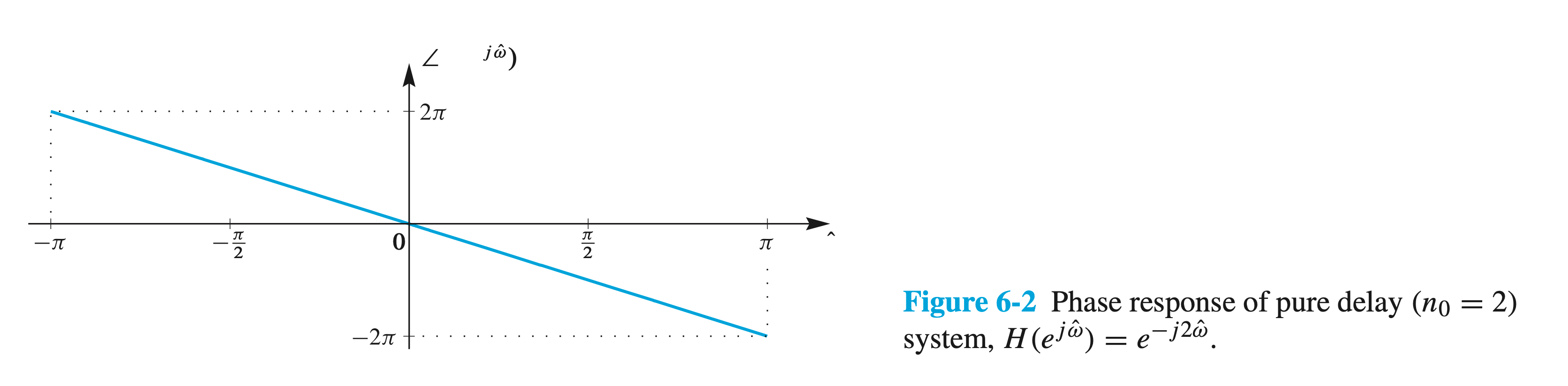
As a result, we can associate the slope of a linear phase versus frequency with time delay as a general rule in all filters.

Since time delay shifts a signal plot horizontally but does not change its shape, we often think of linear phase as an ideal phase response.

First-Difference System

Consider the first-difference system \[ y[n]=x[n]-x[n-1] \] The frequency response of this LTI system is \[ H\left(e^{j \hat{\omega}}\right)=1-e^{-j \hat{\omega}} \]

Since \[ H\left(e^{j \hat{\omega}}\right)=1-(\cos (\hat{\omega})-j \sin (\hat{\omega}))=(1-\cos \hat{\omega})+j \sin \hat{\omega} , \]

the magnitude and phase can be written from the real and imaginary parts \[ \begin{aligned} \left|H\left(e^{j \hat{\omega}}\right)\right| & =\left[(1-\cos \hat{\omega})^2+\sin ^2 \hat{\omega}\right]^{1 / 2} \\ & =[2(1-\cos \hat{\omega})]^{1 / 2}=2|\sin (\hat{\omega} / 2)| \\ \angle H\left(e^{j \hat{\omega}}\right) & =\arctan \left(\frac{\sin \hat{\omega}}{1-\cos \hat{\omega}}\right) \end{aligned} \]

The magnitude and phase in $-3 \pi<\hat{\omega}<3 \pi$ are plotted in Figure 6.3:

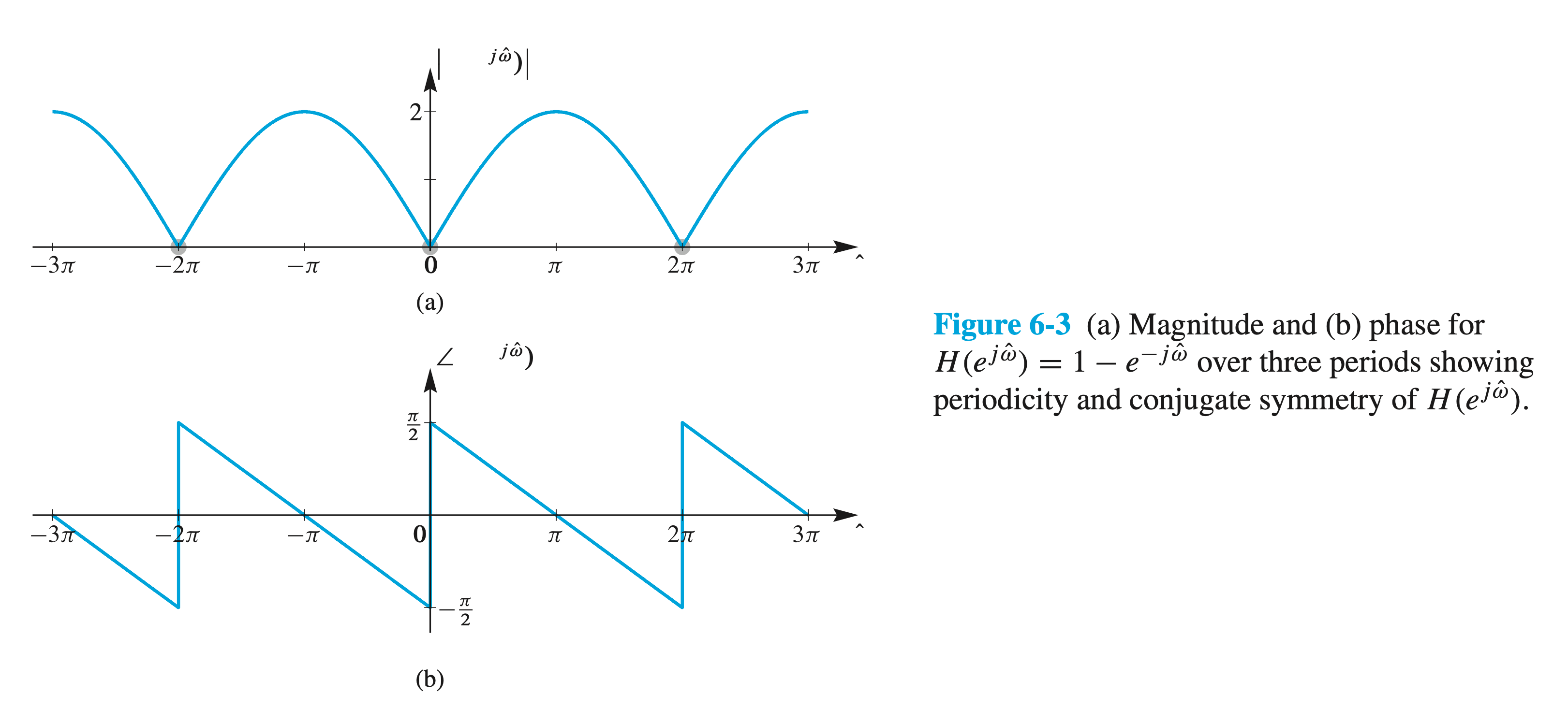
These extended plots allow us to verify that $H\left(e^{j \hat{\omega}}\right)$ is periodic with period $2 \pi$, and to see the conjugatesymmetry properties discussed in Section 6-4.3. Normally, we would plot the frequency response of a discrete-time system only for $-\pi<\hat{\omega} \leq \pi$, or, when there is conjugate symmetry, $0 \leq \hat{\omega} \leq \pi$.

The utility of the magnitude and phase plots of $H\left(e^{j \hat{\omega}}\right)$ can be seen even for this simple example.

In the figure, 6-3 $H\left(e^{j 0}\right)=0$, so we conclude that the system completely removes components with $\hat{\omega}=0$ (i.e., DC).
Furthermore, in the figure(a) we can see that the system boosts components at higher frequencies (near $\hat{\omega}=\pi$ ) relative to the lower frequencies. This sort of filter is called a highpass filter.

The real and imaginary parts and the magnitude and phase can always be derived by standard manipulations of complex numbers. However, there is a simpler approach for getting the magnitude and phase when the sequence of coefficients is either symmetric or antisymmetric about a central point. The following algebraic manipulation of $H\left(e^{j \hat{\omega}}\right)$ is possible because the $\left\{b_k\right\}$ coefficients satisfy the antisymmetry condition: \[ b_k=-b_{M-k} \] where $M=1$ for the first-difference filter. The trick, which we used previously in Example 6-1 on p. 197, is to factor out an exponential whose phase is half of the filter order $(M / 2)$ times $\hat{\omega}$, and then use the inverse Euler formula to combine corresponding positive- and negative-frequency complex exponentials. For the first-difference filter, we exploit (6.18) to write \[ \begin{aligned} H\left(e^{j \hat{\omega}}\right) & =1-e^{-j \hat{\omega}} \\ & =e^{-j \hat{\omega} / 2}\left(e^{j \hat{\omega} / 2}-e^{-j \hat{\omega} / 2}\right) \\ & =2 j e^{-j \hat{\omega} / 2} \sin (\hat{\omega} / 2) \\ & =\underbrace{2 \sin (\hat{\omega} / 2)}_{\text {Magnitude? }} \exp (j \underbrace{(\pi / 2-\hat{\omega} / 2)}_{\text {Phase? }}) \end{aligned} \]

The form derived for $H\left(e^{j \hat{\omega}}\right)$ is almost a valid polar form, but since $\sin (\hat{\omega} / 2)$ is negative for $-\pi<\hat{\omega}<0$, we must write the magnitude as $\left|H\left(e^{j \hat{\omega}}\right)\right|=2|\sin (\hat{\omega} / 2)|$, and then

absorb the negative sign² into the phase response for $-\pi<\hat{\omega}<0$. Thus the correct phase in polar form is \[ \angle H\left(e^{j \hat{\omega}}\right)= \begin{cases}\pi / 2-\hat{\omega} / 2 & 0<\hat{\omega} \leq \pi \\ -\pi+\pi / 2-\hat{\omega} / 2 & -\pi \leq \hat{\omega}<0\end{cases} \]

This formula for the phase is consistent with the phase plot in Fig. 6-3(b), which exhibits several straight line segments, but has discontinuities at $\hat{\omega}=0$ and $\hat{\omega}= \pm 2 \pi$. The size of these discontinuities is $\pi$, since they correspond to sign changes in $H\left(e^{j \hat{\omega}}\right)$.

Example: First-Difference Removes DC

Suppose that the input to a first-difference system is $x[n]=4+2 \cos (0.3 \pi n-\pi / 4)$. Since the output is related to the input by the difference equation $y[n]=x[n]-x[n-1]$, it follows that \[ \begin{aligned} y[n] & =4+2 \cos (0.3 \pi n-\pi / 4)-4-2 \cos (0.3 \pi(n-1)-\pi / 4) \\ & =2 \cos (0.3 \pi n-\pi / 4)-2 \cos (0.3 \pi n-0.55 \pi) \end{aligned} \]

The solution using the frequency-response function is simple.

Since the first-difference system has frequency response \[ H\left(e^{j \hat{\omega}}\right)=2 \sin (\hat{\omega} / 2) e^{j(\pi / 2-\hat{\omega} / 2)} \] the output of this system for the given input can be obtained more quickly via \[ y[n]=4 H\left(e^{j 0}\right)+2\left|H\left(e^{j 0.3 \pi}\right)\right| \cos \left(0.3 \pi n-\pi / 4+\angle H\left(e^{j 0.3 \pi}\right)\right) \]

In other words, we need to evaluate the frequency response only at $\hat{\omega}=0$ and $\hat{\omega}=0.3 \pi$. Since $H\left(e^{j 0}\right)=0$ and \[ \begin{aligned} H\left(e^{j 0.3 \pi}\right) & =2 \sin (0.3 \pi / 2) e^{j(0.5 \pi-0.15 \pi)} \\ & =0.908 e^{j 0.35 \pi} \end{aligned} \] the output is \[ \begin{aligned} y[n] & =(0.908)(2) \cos (0.3 \pi n-\pi / 4+0.35 \pi) \\ & =1.816 \cos (0.3 \pi n+0.1 \pi) \end{aligned} \]

A Simple Lowpass Filter

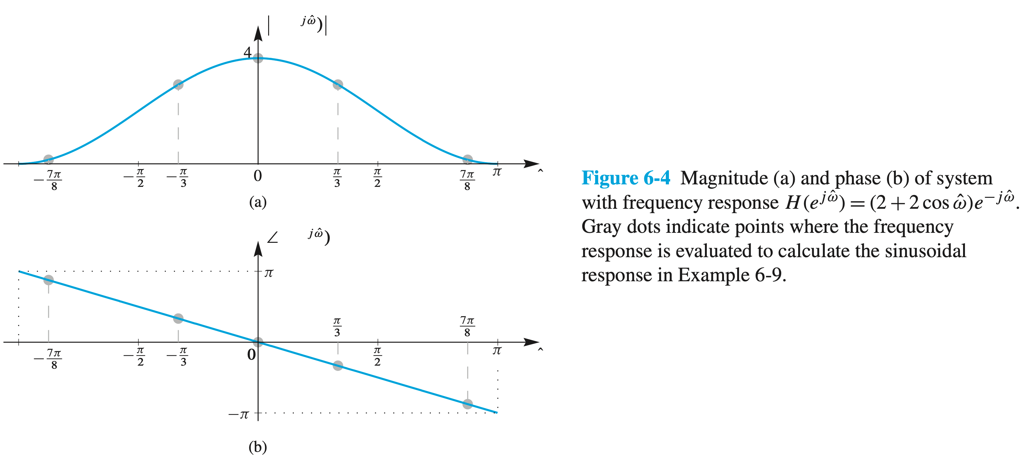
In Examples 6-1, 6-3, and 6-4, the system had frequency response \[ H\left(e^{j \hat{\omega}}\right)=1+2 e^{-j \hat{\omega}}+e^{-j 2 \hat{\omega}}=(2+2 \cos \hat{\omega}) e^{-j \hat{\omega}} \] Since the factor $(2+2 \cos \hat{\omega}) \geq 0$ for all $\hat{\omega}$, it follows that \[ \left|H\left(e^{j \hat{\omega}}\right)\right|=(2+2 \cos \hat{\omega}) \] and \[ \angle H\left(e^{j \hat{\omega}}\right)=-\hat{\omega} \]

These functions are plotted in Fig. 6-4 for $-\pi<\hat{\omega} \leq \pi$.

The phase response (Fig. 6-4(b)) is linear (a straight line) with a slope of -1 , so we know that the system introduces a delay of one sample.

The magnitude response (Fig. 6-4(a)) shows that the system tends to favor the low frequencies (close to $\hat{\omega}=0$ ) with high gain, while it tends to suppress high frequencies (close to $\hat{\omega}=\pi$ ).

Filters with magnitude responses that suppress the high frequencies of the input are called lowpass filters.

Example: Lowpass Filter

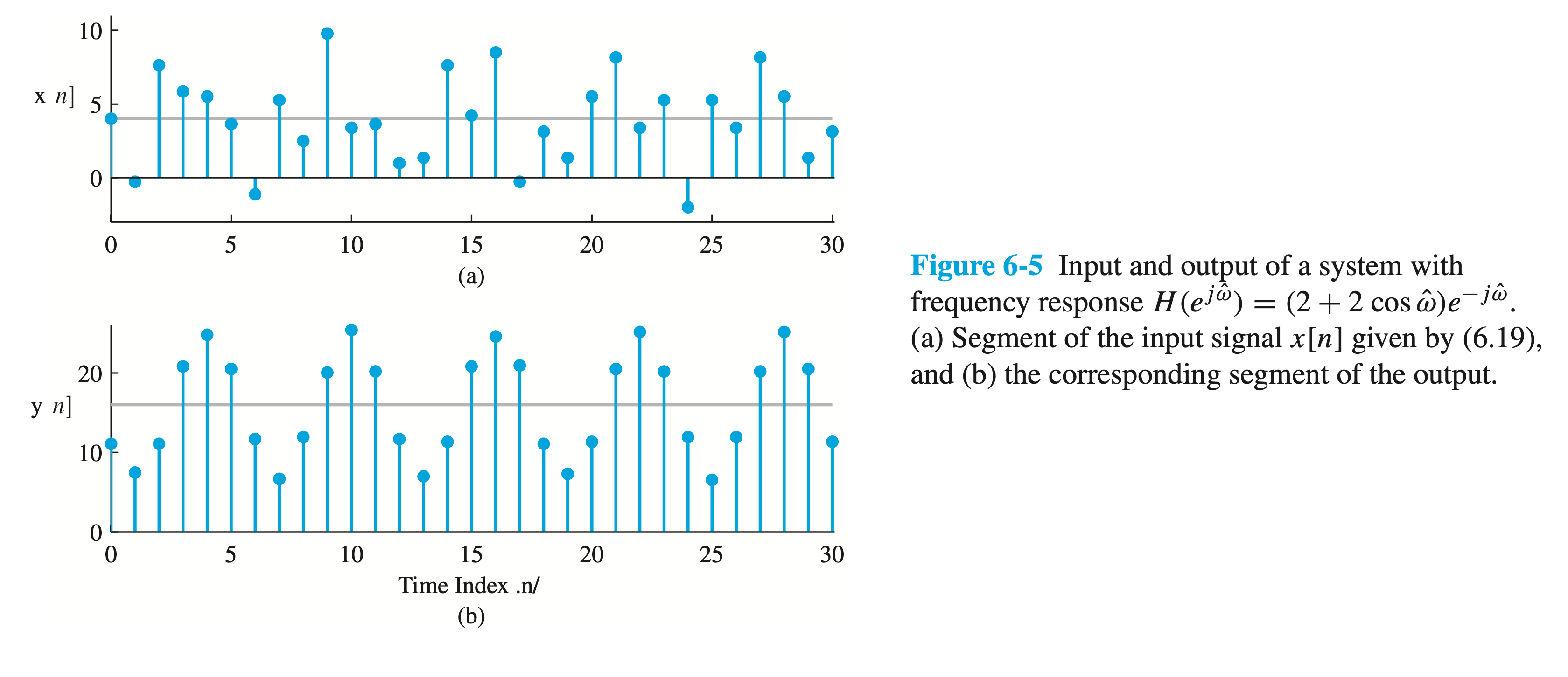
If we repeat Example 6-4, we can show how the plot of $H\left(e^{j \hat{\omega}}\right)$ in Fig. 6-4 makes it easy to find the filter's output for sinusoidal inputs. In Example 6-4, the input was \[ x[n]=4+3 \cos \left(\frac{\pi}{3} n-\frac{\pi}{2}\right)+3 \cos \left(\frac{7 \pi}{8} n\right) \]

as shown in Fig. 6-5(a), and the filter coefficients were $\left\{b_k\right\}=\{1,2,1\}$. In order to get the output signal, we must evaluate $H\left(e^{j \hat{\omega}}\right)$ at frequencies $0, \pi / 3$, and $7 \pi / 8$ giving \[ \begin{aligned} H\left(e^{j 0}\right) & =4 \\ H\left(e^{j \pi / 3}\right) & =3 e^{-j \pi / 3} \\ H\left(e^{j 7 \pi / 8}\right) & =0.1522 e^{-j 7 \pi / 8} \end{aligned} \]

These values are the points indicated with gray dots on the graphs of Fig. 6-4. As in Example 6-4, the output is \[ \begin{aligned} y[n] & =4 \cdot 4+3 \cdot 3 \cos \left(\frac{\pi}{3} n-\frac{\pi}{3}-\frac{\pi}{2}\right)+0.1522 \cdot 3 \cos \left(\frac{7 \pi}{8} n-\frac{7 \pi}{8}\right) \\ & =16+9 \cos \left(\frac{\pi}{3}(n-1)-\frac{\pi}{2}\right)+0.4567 \cos \left(\frac{7 \pi}{8}(n-1)\right) \end{aligned} \]

We can see two features in the output signal $y[n]$. The sinusoid with $\hat{\omega}=7 \pi / 8$ has a very small magnitude because the magnitude response around $\hat{\omega}=\pi$ is relatively small. Also, the linear phase slope of -1 means that the filter introduces a time delay of one sample which is evident in the second and third terms of $y[n]$.

The output of the simple lowpass filter is the time waveform shown in Fig. 6-5(b). Note that the DC component is indicated in both parts of the figure as a gray horizontal line. The output appears to be the sum of a constant level of 16 plus a cosine that has amplitude 9 and seems to be periodic with period 6. Closer inspection reveals that this is not exactly true because there is a third output component at frequency $\hat{\omega}=7 \pi / 8$, which is just barely visible in Fig. 6-5(b). Its size is about 5% of the size of the component with frequency $\hat{\omega}=\pi / 3$.

The gain can be less than or greater than 1 , even though the word suggests greater than.↩︎
Remember that $-1=e^{ \pm j \pi}$, so we can add either $+\pi$ or $-\pi$ to the phase for $-\pi<\hat{\omega}<0$. In this case, we add $-\pi$ so that the resulting phase curve remains between $-\pi$ and $+\pi$ radians for all $\hat{\omega}$.↩︎