Sinusoidal Signals

Posted on 2023-11-21 Edited on 2024-09-17 In Electrical Engineering Views:

Sources:

James McClellan, Ronald Schafer & Mark Yoder. (2015). Sinusoids. DSP First (2nd ed., pp. 9-40). Pearson.

Review of Complex Numbers

Representation

A complex number $z$ may be represented by the notation $z=(x, y)$, where $x,y \in \mathbb R$,

the real part is $x=\Re\{z\}$, and
the imaginary part is $y=\Im \{z\}$.

Note: Electrical engineers use the symbol $j$ for $\sqrt{-1}$ instead of $i$.

We can also represent $z$ as:

Cartesian or rectangular form \[ z=x+j y \]
Polar form: \[ z = r e^{j \theta}=r(\cos \theta+j \sin \theta) \] This is due to the Euler's formula: \[ \begin{equation} \label{eq_Euler's formula} z = r e^{j \theta}=r(\cos \theta+j \sin \theta) \end{equation} \]

Polar form -> Cartesian form: \[ x=r \cos \theta \quad \text { and } \quad y=r \sin \theta \] Cartesian form -> Polar form: \[ r=\sqrt{x^2+y^2} \quad \text { and } \quad \theta=\arctan \left(\frac{y}{x}\right) \]

Magnitude of the complex number

For a complex number $z = e^{j \theta}$, its magnitude, denoted as $|z|$, is: \[ \left|e^{j \theta}\right|=\sqrt{\cos ^2(\theta)+\sin ^2(\theta)}=\sqrt{1}=1 . \] As a result, the magnitude for an arbitary complex number $z = r e^{j \theta}$ is $|z| = r$.

Complex conjugate

The complex conjugate of a complex number is the number with an equal real part and an imaginary part equal in magnitude but opposite in sign. The complex conjugate of $z$ is often denoted as $\bar{z}$ or $z^*$.

In cartesian or rectangular form: \[ z^* = x - jy . \]
In polar form: \[ z^* = r e^{- j \theta}=r(\cos \theta - j \sin \theta) \]

Complex Plane

Complex numbers are often represented as points in a complex plane, where the real and imaginary parts are the horizontal and vertical coordinates, respectively, as shown in the figure:

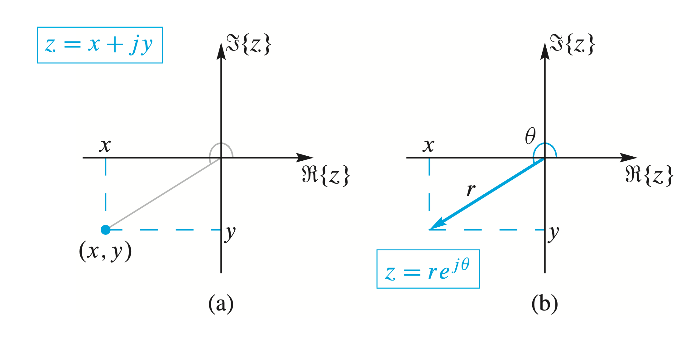
$r$: the length of the vector. Also called the magnitude of $z$ (denoted $|z|$),
$\theta$: the angle of the vector. Also called the argument of $z$ (denoted $\arg z$).

Inverse Euler Formulas

The inverse Euler formulas allow us to write the cosine function in terms of complex exponentials as \[ \begin{equation} \label{eq2.2.1} \cos \theta=\frac{e^{j \theta}+e^{-j \theta}}{2} \end{equation} \] and also the sine function can be expressed as \[ \begin{equation} \label{eq2.2.2} \sin \theta=\frac{e^{j \theta}-e^{-j \theta}}{2 j} \end{equation} \]

Equation $\eqref{eq2.2.1}$ can be used to express $\cos \left(\omega_0 t+\varphi\right)$ in terms of two complex exponentials as follows: \[ \begin{aligned} A \cos \left(\omega_0 t+\varphi\right) & =A\left(\frac{e^{j\left(\omega_0 t+\varphi\right)}+e^{-j\left(\omega_0 t+\varphi\right)}}{2}\right) \\ & =\frac{1}{2} X e^{j \omega_0 t}+\frac{1}{2} X^* e^{-j \omega_0 t} \\ & =\frac{1}{2} z(t)+\frac{1}{2} z^*(t) \\ & =\Re\{z(t)\} \end{aligned} \] where $*$ denotes complex conjugation.

Sinusoidal signals

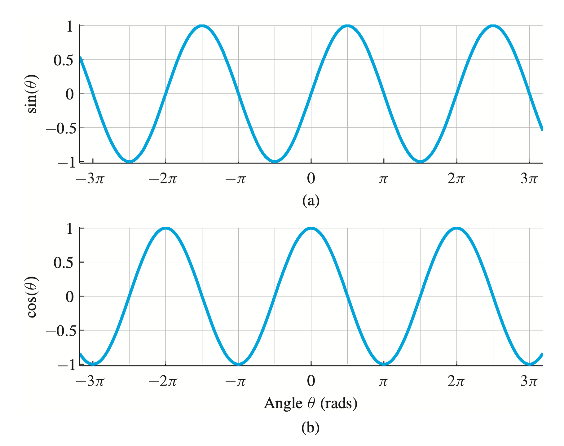Figure 2.5 (a) Sine function and (b) cosine function plotted versus angle θ. Both functions have a period of 2π.

Many physical systems generate signals that can be modeled (i.e., represented mathematically) as sine/cosine functions versus time:

\[ \begin{equation} \label{1.1} x(t)=A \cos \left(\omega_0 t+\varphi\right) \end{equation} \] (Note that $\sin$ <==> $\cos$)

$A$: Amplitude.
$\omega_0$: Radian frequency.
- $ω_0$ must have units of rad/s if $t$ has units of seconds.
- Similarly, $f_0 = \frac{ω_0}{2π}$ is called the cyclic frequency, and $f_0$ must have units of $s^{−1}$, or hertz(abbreviated Hz).
$\varphi$: Phase.

Note: Angles can be specified in degrees ($^{\circ}$) or radians ($\text{rad}$).

In Signal Processing, this signal is called: cosine/sin signal or cosine/sine wave or sinusoidal signal or sinusoid.

In the latter section, we will see that a sinusoidal signal is the real part of a more general complex exponential signal.

$T_0$: the period of the sinusoid. It's the time duration of one cycle of the sinusoid: \[ x(t) = x(t+T_0) . \]

Relation of frequency($w_0$ or $f_0$) to period $T_o$: \[ T_0 = \frac {2π}{w_0} = \frac {2π}{2π f_0} = \frac {1}{f_0} . \]

phase and time shift: whenever a signal can be expressed in the form \[ x_1(t)=s\left(t-t_1\right) \] , we say that $x_1(t)$ is a time-shifted version of $s(t)$.
1. If $t_1 > 0$, the signal $s(t)$ has been delayed in time.
2. If $t_1 < 0$, the signal $s(t)$ has been advanced in time.
Note that: \[ \begin{aligned} x_0\left(t-t_1\right) & =A \cos \left(\omega_0\left(t-t_1\right)\right) \end{aligned} \]

Sampling and Plotting Sinusoids

Sinusoidals are continuous funtions, but computers can only deal with discrete signals.

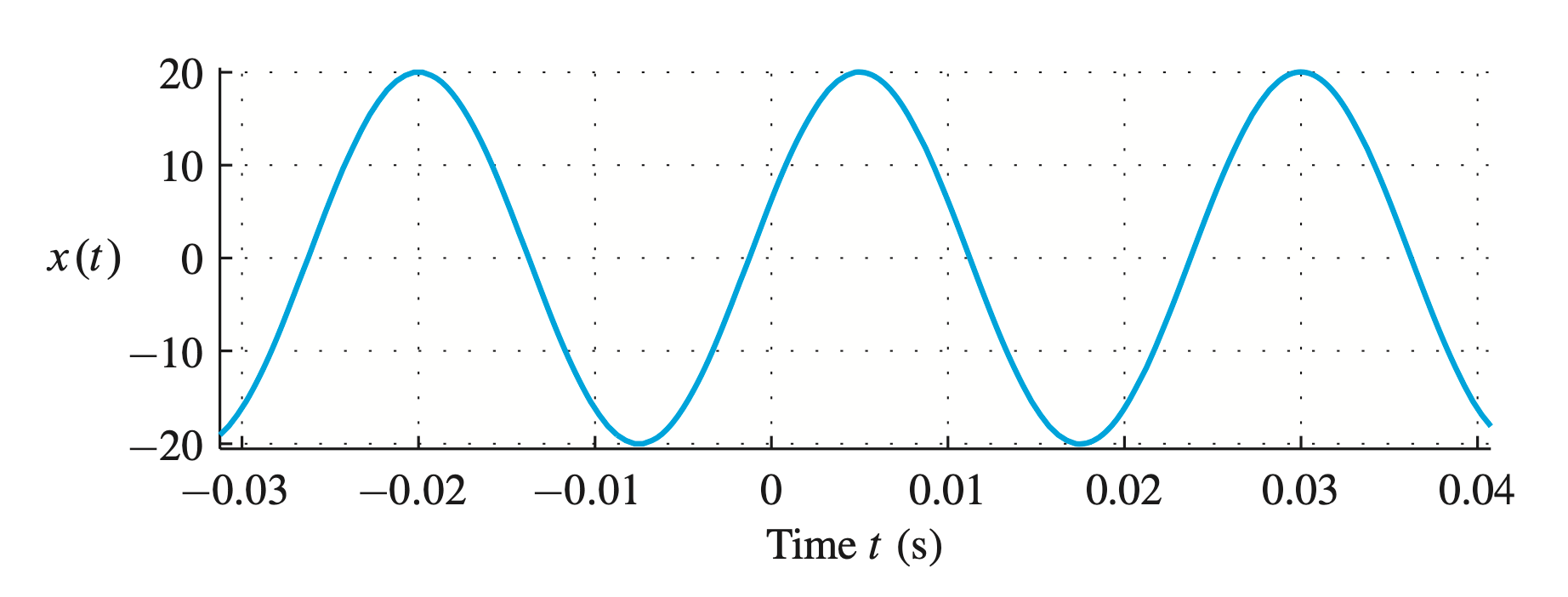
For example, if we wish to plot a function such as \[ x(t)=20 \cos (2 \pi(40) t-0.4 \pi) \] with parameters: $A = 20$, $ω_0 = 2π(40)$, $f_0 = 40$ Hz, and $φ = −0.4π$ rad.

which is shown in above figure, we must evaluate $x(t)$ at a discrete set of times. Usually we pick a uniform set $t_n=n T_s$, where $n$ is an integer. Then from $x(t)$ we obtain the sequence of samples \[ x\left(n T_s\right)=20 \cos \left(80 \pi n T_s-0.4 \pi\right) \] where $T_s$ is called the sample spacing or sampling period.

Complex exponential signals

Using Euler's formula $\eqref{eq_Euler's formula}$, the complex exponential signal is defined as \[ \begin{align} z(t) & =A e^{j\left(\omega_0 t+\varphi\right)} \label{eq3.1} \\ & = A \cos \left(\omega_0 t+\varphi\right)+j A \sin \left(\omega_0 t+\varphi\right) \end{align} \]

the magnitude is always a positive constant (i.e., $|z(t)|=A$ )
the angle is $\arg z(t)=\left(\omega_0 t+\varphi\right)$.
A sinusoidal signal $\eqref{eq1.1}$ is the real part of a complex exponential signal $\eqref{eq3.1}$ \[ x(t)=\Re\left\{A e^{j\left(\omega_0 t+\varphi\right)}\right\}=A \cos \left(\omega_0 t+\varphi\right) \]

The usage of complex exponential signal is that it is a alternative representation for the real cosine signal.

The Rotating Phasor Interpretation

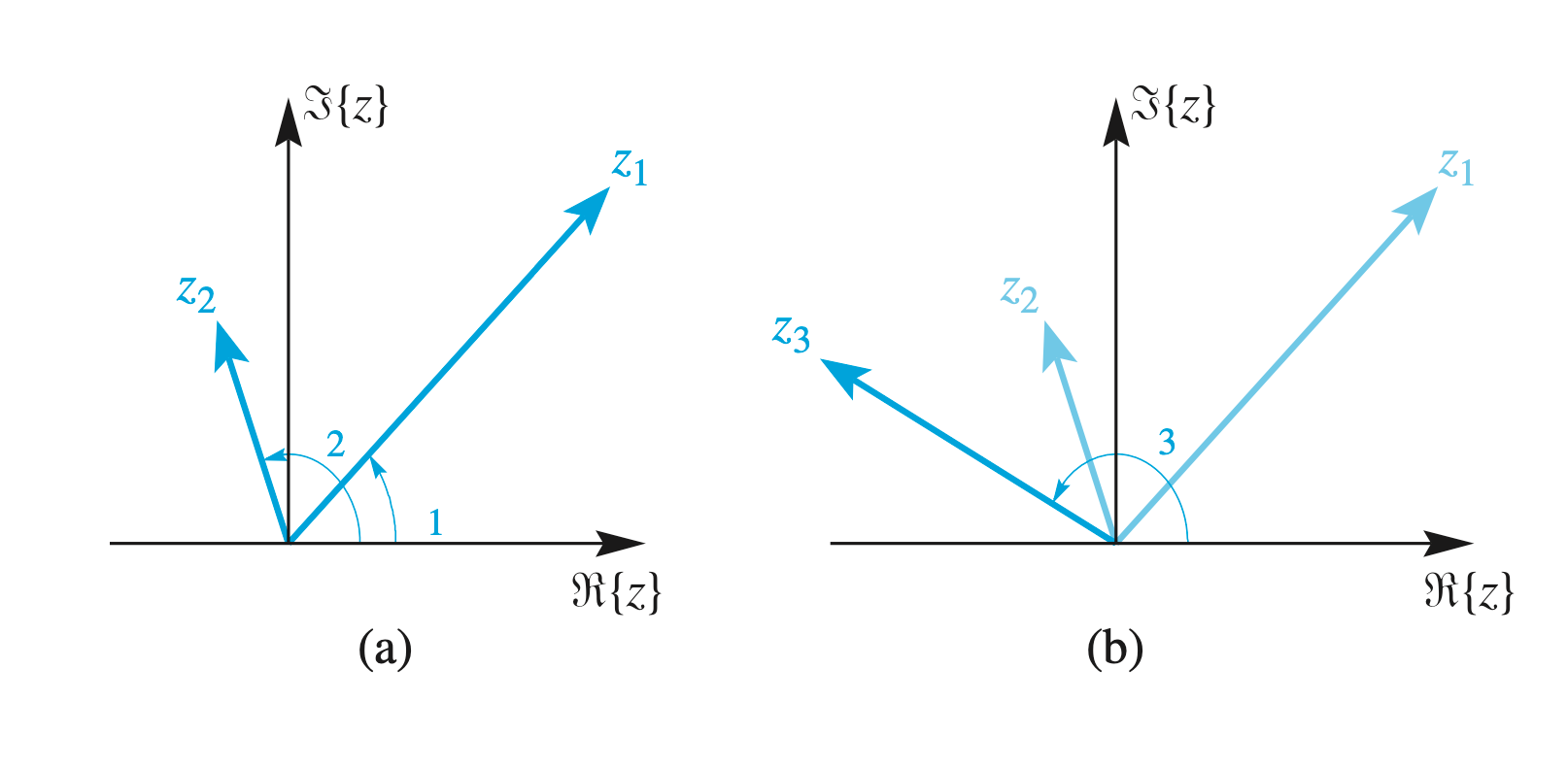
Geometric view of complex multiplication

Consider $z_3=z_1 z_2$, where $z_1=r_1 e^{j \theta_1}$ and $z_2=r_2 e^{j \theta_2}$.

Then the multiplication \[ z_3=z_1 z_2 \]

is \[ z_3=r_1 e^{j \theta_1} r_2 e^{j \theta_2}=r_1 r_2 e^{j \theta_1} e^{j \theta_2}=\overbrace{r_1 r_2}^{r_3} e^{j(\overbrace{\theta_1+\theta_2}^{\theta_3}} \] Geometric view: From the above figure, $z_3$ is a rotated and scaled version of $z_2$ because $\angle z_3=\angle z_2+\theta_1$, and the length of $z_3$ is $r_1$ times the length of $z_2$. Here, $r_1=1.72, r_2=0.77$, and $r_3=1.32$.

Hense, complex multiplication involves rotation and scaling.

Thus, the complex exponential signal is interpreted as a complex vector that rotates as time increases. If we use $A$ and $\varphi$ to define a complex number: \[ X=A e^{j \varphi} \] then the complex exponential $\eqref{eq3.1}$ can be expressed as \[ z(t)=X e^{j \omega_0 t} = A e^{j \varphi} e^{j \omega_0 t}=A e^{j \theta(t)} \] (i.e., $z(t)$ is the product of the complex constant $X$ and the complex-valued time function $e^{j \omega_0 t}$ ).

where $\theta(t)$ is a time-varying angle function \[ \theta(t)=\omega_0 t+\varphi \quad(\text { radians }) \]

Phaser Addition

Theorem: a sum of $N$ cosine signals of differing amplitudes and phases, but with the same frequency, can always be reduced to a single cosine signal of the same frequency. \[ \begin{align} x(t) &= \sum_{k=1}^N A_k \cos \left(\omega_0 t+\varphi_k\right) \label{eq4.1} \\ & = A \cos \left(\omega_0 t+\varphi\right) \nonumber \end{align} \]

A very simple proof can be based on the complex exponential representation of the cosine signals.

Proof

Proof using complex exponential representation:

First, any sinusoid can be written in the form: \[ A \cos \left(\omega_0 t+\varphi\right)=\Re\left\{A e^{j\left(\omega_0 t+\varphi\right)}\right\}=\Re\left\{A e^{j \varphi} e^{j \omega_0 t}\right\} . \] For any set of complex numbers $\left\{X_k\right\}$, the sum of the real parts is equal to the real part of the sum, so we have \[ \Re\left\{\sum_{k=1}^N X_k\right\}=\sum_{k=1}^N \Re\left\{X_k\right\} . \] Then we pick a $A e^{j \varphi}$ that satisfies \[ \begin{equation} \label{eq4.3} \sum_{k=1}^N A_k e^{j \varphi_k}= A e^{j \varphi} . \end{equation} \]

Therefore, $$ \[\begin{align} & \sum_{k=1}^N A_k \cos \left(\omega_0 t+\varphi_k\right) \\ = & \sum_{k=1}^N \Re\left\{A_k e^{j\left(\omega_0 t+\varphi_k\right)}\right\} \label{eq4.4.1} \\ = & \Re\left\{\sum_{k=1}^N A_k e^{j \varphi_k} e^{j \omega_0 t}\right\} \nonumber \\ = & \Re\left\{\left(\sum_{k=1}^N A_k e^{j \varphi_k}\right) e^{j \omega_0 t}\right\} \label{eq4.4.3} \\ = & \Re\left\{\left(A e^{j \varphi}\right) e^{j \omega_0 t}\right\}=\Re\left\{A e^{j\left(\omega_0 t+\varphi\right)}\right\} \label{eq4.4.4} \\ = & A \cos \left(\omega_0 t+\varphi\right) . \nonumber \end{align}\] $$

The equality of $\eqref{eq4.4.1}$ is due to Euler's formula $\eqref{eq_Euler's formula}$.
The transition from $\eqref{eq4.4.3}$ to $\eqref{eq4.4.4}$ is due to $\eqref{eq4.3}$.