Stationary Stochastic Processes and Markov Chains

1. EE 376A: Information Theory. Winter 2018. Lecture 4. - Stanford University
2. EE 376A: Information Theory. Winter 2017. Lecture 4. - Stanford University
3. Elements of Information Theory

Stochastic Process

Definition: A stochastic process $\left\{X_i\right\}$ is an indexed sequence of random variables. In general, there can be an arbitrary dependence among the random variables.

The process is characterized by the joint probability mass functions $$\mathrm{Pr}\{(X_1,X_2,\dots ,X_n)=(x_1,x_2,\dots ,x_n)\}=p(x_1,x_2,\dots ,x_n).$$ with $(x_1,x_2,\dots ,x_n)\in {\mathcal{X}}^n$ for $n=1,2,\dots$

Stationary Stochastic Process

Definition: A stochastic process is said to be stationary if the joint distribution of any subset of the sequence of random variables is invariant with respect to shifts in the time index; that is, $$\begin{array}{rl}& \mathrm{Pr}\{X_1=x_1,X_2=x_2,\dots ,X_n=x_n\}\\ & =\mathrm{Pr}\{X_{1+l}=x_1,X_{2+l}=x_2,\dots ,X_{n+l}=x_n\}\end{array}$$ for every $n$ and every shift $l$ and for all $x_1,x_2,\dots ,x_n\in \mathcal{X}$.

Markov Chain

A Markov process or a Markov chain is a stochastic process indexed by time, and with the property that the future is independent of the past, given the present.

Markov processes, named for Andrei Markov, are among the most important of all random processes. In a sense, they are the stochastic analogs of differential equations and recurrence relations, which are of course, among the most important deterministic processes.

Source: Introduction to Markov Processes.

本文只讨论时间和状态空间均为离散的情况的markov chain.

Definition: A discrete stochastic process $X_1,X_2,\dots$ is said to be a Markov chain or a Markov process if for $n=1,2,\dots$, $$\begin{array}{rl}\mathrm{Pr}(X_{n+1}& =x_{n+1}\mid X_n=x_n,X_{n-1}=x_{n-1},\dots ,X_1=x_1)\\ & =\mathrm{Pr}(X_{n+1}=x_{n+1}\mid X_n=x_n)\end{array}$$ for all $x_1,x_2,\dots ,x_n,x_{n+1}\in \mathcal{X}$.

We can denote them as $X_1\to X_2\to \cdots \to X_n$.

• Note: If there're only two r.v. s, say $X_1$ and $X_2$. They must form a Markov chain $X_1{X}_2$, or $X_2\to X_1$ since Markov chain is invertable(->Proof). Because $$P(X_1|X_2,\text{there's no more}{X}_i)=P(X_1|X_2)$$

PMF of a Markov Chain

The joint probability mass function of the random variables can be written as $$p(x_1,x_2,\dots ,x_n)=p\left(x_1\right)p(x_2\mid x_1)p(x_3\mid x_2)\cdots p(x_n\mid x_{n-1}).$$

Proof

let's prove this expression with mathematical induction:

1. Base Case (n = 2): $$p(x_1,x_2)=p(x_1)p(x_2\mid x_1)p(x_1,x_2)=p(x_1)p(x_2\mid x_1).$$

2. Inductive Step: Assume the expression holds for $n=k$: $$p(x_1,x_2,\dots ,xk)=p(x_1)p(x_2\mid x_1)p(x_3\mid x_2)\cdots p(x_k\mid x_{k-1}).$$

3. Now, consider $n=k+1$: $$\begin{array}{rl}p(x_1,x_2,\dots ,x_{k+1})& =p(x_1,x_2,\cdots ,x_k)p(x_{k+1}\mid x_1,x_2,\cdots ,x_k)\\ & =p(x_1,x_2,\cdots ,x_k)p(x_{k+1}\mid x_k)\\ & =p(x_1)p(x_2\mid x_1)p(x_3\mid x_2)\cdots p(x_k\mid x_{k-1})\end{array}$$

   • In the second line we apply $p(x_{k+1}\mid x_1,x_2,\cdots ,x_k)=p(x_{k+1}\mid x_k)$, which is the preperty of a Markov chain.
   • In third line we apply our assumtion in the aductive step.

4. This expression matches the assumed expression for $n=k$. Therefore, by mathematical induction, the expression holds for all $n$.

   Hence, the joint probability mass function of the Markov chain can be written as:

Time Invariant

Definition: The Markov chain is said to be time invariant if the conditional probability $p(x_{n+1}\mid x_n)$ does not depend on $n$; that is, for $n=$ $1,2,\dots$, $$\mathrm{Pr}\{X_{n+1}=b\mid X_n=a\}=\mathrm{Pr}\{X_2=b\mid X_1=a\}\text{ for all }a,b\in \mathcal{X}.$$

We will assume that the Markov chain is time invariant unless otherwise stated.

If $\left\{X_i\right\}$ is a Markov chain, $X_n$ is called the state at time $n$.

A time invariant Markov chain is characterized by its initial state and a probability transition matrix $P=\left[P_{ij}\right],i,j\in \{1,2,\dots ,m\}$, where $P_{ij}=\mathrm{Pr}\{X_{n+1}=$ $j\mid X_n=i\}$.

If it is possible to go with positive probability from any state of the Markov chain to any other state in a finite number of steps, the Markov chain is said to be irreducible. If the largest common factor of the lengths of different paths from a state to itself is 1 , the Markov chain is said to aperiodic.

Properties

If random variables $X,Y,Z$ form a Markov chain (denoted by $X\to Y\to Z$ ), their PMF satisfies: $$\begin{array}{}\text{(1)}& p(x,y,z)=p(x)p(y\mid x)p(z\mid y).\end{array}$$

• $X\to Y\to Z$ implies that $Z\to Y\to X$. Thus, the condition is sometimes written $X\leftrightarrow Y\leftrightarrow Z$.
• If $Z=f(Y)$, then $X\to Y\to Z$.

Conditionally Independence

$X\to Y\to Z$ <==> $X$ and $Z$ are conditionally independent given $Y$: $p(x,z|y)=p(x|y)p(z|y)$. Proof:

Proof

==>

Given $X\to Y\to Z$, we have $p(x,z|y)=p(x|y)p(z|y)$.

Proof: $$\begin{array}{}\text{(2)}& p(x,z\mid y)& =\frac{p(x,y,z)}{p(y)}\text{(3)}& & =\frac{p(x)p(y\mid x)p(z\mid y)}{p(y)}\text{(4)}& & =\frac{p(x,y)p(z\mid y)}{p(y)}\text{(5)}& & =p(x\mid y)p(z\mid y).\end{array}$$ $\text{(2)}$: the definition of conditional probability.

$\text{(3)}$: from $\text{(1)}$.

$\text{(4)}$: the definition of conditional probability: $p(x)p(y|x)=p(x,y)$.

$\text{(5)}$: the definition of conditional probability: $\frac{p(x,y)}{p(y)}=p(x\mid y)$.

---

<==

Given $p(x,z|y)=p(x|y)p(z|y)$, we have $X\to Y\to Z$, which means $\text{(1)}$.

Proof: we just need to inverse the above proof: $$p(x|y)p(z|y)=\frac{p(x,y)p(z\mid y)}{p(y)}=\frac{p(x)p(y\mid x)p(z\mid y)}{p(y)}$$ And we know that: $$p(x,z\mid y)=\frac{p(x,y,z)}{p(y)}.$$ Since $$p(x,z|y)=p(x|y)p(z|y)$$ Then: $$\frac{p(x)p(y\mid x)p(z\mid y)}{p(y)}=\frac{p(x,y,z)}{p(y)},$$ which means $\text{(1)}$.

Data Processing Inequality

Theorem(Data-processing inequality): If $X\to Y\to Z$, then $I(X;Y)\ge I(X;Z)$.

Proof:

By the chain rule, we can expand mutual information in two different ways: $$\begin{array}{rl}I(X;Y,Z)& =I(X;Z)+I(X;Y\mid Z)\\ & =I(X;Y)+I(X;Z\mid Y).\end{array}$$

Since $X$ and $Z$ are conditionally independent given $Y$, we have $I(X;Z\mid Y)=0$.

Since $I(X;Y\mid Z)\ge 0$, we have $$I(X;Y)\ge I(X;Z).$$

We have equality if and only if $I(X;Y\mid Z)=0$ (i.e., $X\to Z\to Y$ forms a Markov chain). Similarly, one can prove that $I(Y;Z)\ge I(X;Z)$.

Corollary

Corollary: In particular, if $Z=g(Y)$, we have $I(X;Y)\ge I(X;g(Y))$. Proof: $X\to Y\to g(Y)$ forms a Markov chain. Thus functions of the data $Y$ cannot increase the information about $X$. Corollary If $X\to Y\to Z$, then $I(X;Y\mid Z)\le I(X;Y)$.

Proof

Proof: We note in $\text{(???)}$ and $\text{(???)}$ that $I(X;Z\mid Y)=0$, by Markovity, and $I(X;Z)\ge 0$. Thus, $$I(X;Y\mid Z)\le I(X;Y).$$

Thus, the dependence of $X$ and $Y$ is decreased (or remains unchanged) by the observation of a "downstream" random variable $Z$. Note that it is also possible that $I(X;Y\mid Z)>I(X;Y)$ when $X,Y$, and $Z$ do not form a Markov chain. For example, let $X$ and $Y$ be independent fair binary random variables, and let $Z=X+Y$. Then $I(X;Y)=0$, but $$\begin{array}{rl}I(X;Y\mid Z)& =H(X\mid Z)-H(X\mid Y,Z)\\ & =H(X\mid Z)\\ & =P(Z=1)H(X\mid Z=1)\\ & =\frac{1}{2}\end{array}$$ bit.

Stationary Distribution

If the probability mass function of the random variable at time $n$ is $p\left(x_n\right)$, the probability mass function at time $n+1$ is $$p\left(x_{n+1}\right)=\sum _{x_n}p\left(x_n\right)P_{x_n{x}_{n+1}}.$$

A distribution on the states such that the distribution at time $n+1$ is the same as the distribution at time $n$ is called a stationary distribution.

Stationary distribution is so called because if the initial state of a Markov chain is drawn according to a stationary distribution, the Markov chain forms a stationary process.

If the finite-state Markov chain is irreducible and aperiodic, the stationary distribution is unique, and from any starting distribution, the distribution of $X_n$ tends to the stationary distribution as $n\to \mathrm{\infty }$. (//TO BE PROVED)

Example: Mickey Mouse Markov Chain

We consider an example of two-state Markov chain, which we call Mickey Mouse Markov Chain [MMMC], in order to understand basic properties of Markov chains.

Mickey Mouse Markov Chain

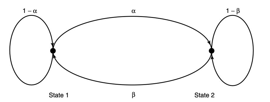
The probability transition matrix of MMMC is: $$P=\left[\begin{array}{cc}1-\alpha & \alpha \\ \beta & 1-\beta \end{array}\right]$$ Let the stationary distribution be represented by a vector $\mu$ whose components are the stationary probabilities of states 1 and 2 , respectively.

//Can't understand:

Then the stationary probability can be found by solving the equation $\mu P=\mu$ or, more simply, by balancing probabilities.

For the stationary distribution, the net probability flow across any cut set in the state transition graph is zero. Applying this to Figure 4.1, we obtain $${\mu }_1\alpha ={\mu }_2\beta$$

Since ${\mu }_1+{\mu }_2=1$, the stationary distribution is $${\mu }_1=\frac{\beta }{\alpha +\beta },{\mu }_2=\frac{\alpha }{\alpha +\beta }.$$

If the Markov chain has an initial state drawn according to the stationary distribution, the resulting process will be stationary. The entropy of the

state $X_n$ at time $n$ is $$H\left(X_n\right)=H(\frac{\beta }{\alpha +\beta },\frac{\alpha }{\alpha +\beta }).$$

However, this is not the rate at which entropy grows for $H(X_1,X_2,\dots$, $X_n)$. The dependence among the $X_i$ 's will take a steady toll.