Asymptotic Equipartition Property
Sources:
- EE 376A: Information Theory. Winter 2018. Lecture 4. - Stanford University
- EE 376A: Information Theory. Winter 2017. Lecture 4. - Stanford University
- Elements of Information Theory
Intro
In information theory, the analog of the law of large numbers(LLN) is the asymptotic equipartition property (AEP).
It is a direct consequence of the weak law of large numbers.
The law of large numbers states that for iid random variables, \(\frac{1}{n} \sum_{i=1}^n X_i\) is close to its expected value \(E(X)\) for large values of \(n\).
The AEP states that \(\frac{1}{n} \log \frac{1}{p\left(X_1, X_2, \ldots, X_n\right)}\) is close to the entropy \(H\), where \(X_1, X_2, \ldots, X_n\) are i.i.d. random variables and \(p\left(X_1, X_2, \ldots, X_n\right)\) is the probability of observing the sequence \(X_1, X_2, \ldots, X_n\). Thus, the probability \(p\left(X_1, X_2, \ldots, X_n\right)\) assigned to an observed sequence will be close to \(2^{-n H}\) \[ \begin{aligned} \frac{1}{n} \log \frac{1}{p\left(X_1, X_2, \ldots, X_n\right)} \rightarrow H \\ p\left(X_1, X_2, \ldots, X_n\right) \rightarrow 2^{-nH} \end{aligned} \]
This enables us to divide the set of all sequences into two sets, the typical set, where the sample entropy is close to the true entropy, and the nontypical set, which contains the other sequences.
Most of our attention will be on the typical sequences. Any property that is proved for the typical sequences will then be true with high probability and will determine the average behavior of a large sample.
Notation
Memoryless source: \(X_1, X_2, \ldots\) iid \(\sim X\), where \(X\) denotes one PMF of arbitory \(X_i\). Note that "memoryless" is used here because samples are drawn iid and have no dependence on past realizations.
- Note: All i.i.d. r.v. have the same probability distribution and the same entropy.
Alphabet: \(\mathcal{X}=\{1,2, \ldots, r\}\) specifies the possible values that each symbol \(X_i\) can take on. The size of \(\mathcal{X}\) is denoted \(|\mathcal{X}|\).
Source sequence: \(X^n=\left(X_1, \ldots, X_n\right)\) denotes the \(n\)-tuple that specifies a sequence of \(n\) source symbols. In other words, \(X^n\) is a stochastic process. Further note that \(\mathcal{X}^n\) indicates the set of all possible source sequences of length \(n\).
- Since the source symbols are memoryless here. \(X^n\) is an iid stochastic process. It's also denoted as \(\left\{X_i\right\}\) in some literatures.
Probability of \(X^n\) where \(X_i\) are i.i.d. : The probability assigned to a source sequence \(X^n\) is given by \(P\left(X^n\right)=\prod_{i=1}^n P_{\mathcal{X}}\left(X_i\right)\). Since we implicitly evaluate the probabilities over the alphabet \(\mathcal{X}\), we may also omit \(\mathcal{X}\) amd write \[ \begin{equation} \label{eq1} P\left(X^n\right)=\prod_{i=1}^n P\left(X_i\right) . \end{equation} \]
The \(\epsilon\)-typical Set
Definition: For some \(\epsilon>0\), the source sequence \(X^n\) is \(\epsilon\)-typical if, \[ \begin{equation} \label{eq2} \left|-\frac{1}{n} \log P\left(X^n\right)-H(X)\right| \leq \epsilon . \end{equation} \]
Let \(A_\epsilon^{(n)}\) denote the " \(\epsilon\)-typical set", that is the set of all source sequences \(X^n\) that are \(\epsilon\)-typical.
即: \(X^n \in A_\epsilon^{(n)}\) <==> \(X^n\) is an \(\epsilon\)-typical set <==> \(\left|-\frac{1}{n} \log P\left(X^n\right)-H(X)\right| \leq \epsilon\).
Furthermore, note the following equivalent ways of defining \(\epsilon\)-typicality:
- \(\eqref{eq2}\)
- \[ \begin{align} & \quad H(X)-\epsilon \nonumber \\ \leq & \quad -\frac{1}{n} \log P\left(X^n\right) \label{eq2.1} \\ \leq & \quad H(X)+\epsilon \nonumber \end{align} \]
- \[ \begin{align} & \quad -n(H(X)+\epsilon \nonumber \\ \leq & \quad \log \left(P\left(X^n\right)\right) \label{eq2.2} \\ \leq & \quad -n(H(X)-\epsilon) \nonumber \end{align} \]
- \[ \begin{align} & \quad 2^{-n(H(X)+\epsilon)} \nonumber \\ \leq & \quad P\left(X^n\right) \label{eq2.3} \\ \leq & \quad 2^{-n(H(X)-\epsilon)} \nonumber \end{align} \]
We have \(\eqref{eq2}\) <==> \(\eqref{eq2.1}\) <==> \(\eqref{eq2.2}\) <==> \(\eqref{eq2.3}\).
From \(\eqref{eq2.3}\) we can say that every \(\epsilon\)-typical set has probability roughly \(2^{-n H(X)}\).
Theorem: \(P\left(X^n \in A_\epsilon^{(n)}\right) \approx 1\)
Theorem: \(\forall \epsilon>0, P\left(X^n \in A_\epsilon^{(n)}\right) \stackrel{n \rightarrow \infty}{\longrightarrow} 1\).
Proof
Note that \(X^n \in A_\epsilon^{(n)}\) <==> \(X^n\) is an \(\epsilon\)-typical set <==> \(\left|-\frac{1}{n} \log P\left(X^n\right)-H(X)\right| \leq \epsilon\). So we have \[ P\left(X^n \in A_\epsilon^{(n)}\right) = P\left(\left|-\frac{1}{n} \log P\left(X^n\right)-H(X)\right| \leq \epsilon\right) \]
Also, we know that \(P\left(X^n\right)=\prod_{i=1}^n P\left(X_i\right)\). Then the right term can be reformed to \[ P\left(\left|-\frac{1}{n} \log \left[\prod_{i=1}^n P\left(X_i\right)\right]-H(X)\right| \leq \epsilon\right) . \] By \(\eqref{eq1}\), it then can be reformed to \[ P\left(\left|\frac{1}{n} \sum_{i=1}^n \log \frac{1}{P\left(X_i\right)}-H(X)\right| \leq \epsilon\right) \] As a result, we have \[ P\left(X^n \in A_\epsilon^{(n)}\right) = P\left(\left|\frac{1}{n} \sum_{i=1}^n \log \frac{1}{P\left(X_i\right)}-H(X)\right| \leq \epsilon\right) . \]
Note that since \(X_i\) are iid, \(\log \frac{1}{P\left(X_i\right)}\) are iid. Then by the weak law of large numbers (LLN), \[ P\left(\left|\frac{1}{n} \sum_{i=1}^n \log \frac{1}{P\left(X_i\right)}- E\left(\log \frac{1}{P(X)}\right)\right| \leq \epsilon\right) \stackrel{n \rightarrow \infty}{\longrightarrow} 1 . \] Here we just treat \(\log \frac{1}{P\left(X_i\right)}\) as iid r.v, then apply the LLN.
Recalling that by the definition of entrypy, \(H(X) \triangleq E\left(\log \frac{1}{P(X)}\right)\), so \[ P\left(\left|\frac{1}{n} \sum_{i=1}^n \log \frac{1}{P\left(X_i\right)}- H(X)\right| \leq \epsilon\right) \stackrel{n \rightarrow \infty}{\longrightarrow} 1 . \] To conclude,
\[ P\left(X^n \in A_\epsilon^{(n)}\right)=P\left(\left|\frac{1}{n} \sum_{i=1}^n \log \frac{1}{P\left(X_i\right)}-H(X)\right| \leq \epsilon\right) \stackrel{n \rightarrow \infty}{\longrightarrow} 1 . \]
Note: Since \(P\left(X^n \in A_\epsilon^{(n)}\right) \approx 1\) and \(A_\epsilon^{(n)}\) is comprised of sequences each with probability roughly \(2^{-n H(X)}\) of being observed(See \(\eqref{eq2.3}\)), then \(\left|A_\epsilon^{(n)}\right| \approx 2^{n H(X)}\). We'll provide more rigorous bounds on \(\left|A_\epsilon^{(n)}\right|\) in the following theorem.
AEP
From Theorem: \(P\left(X^n \in A_\epsilon^{(n)}\right) \approx 1\), we know that for any \(\epsilon>0\), the probabilistic mass in \(\mathcal{X}^n\) is almost entirely concentrated in \(A_\epsilon^{(n)}\).
From \(\eqref{eq2}\), we know that if \(X^n \in A_\epsilon^{(n)}\), then for a fixed(given in \(A_\epsilon^{(n)}\)) \(\epsilon>0\), we have \(\left|-\frac{1}{n} \log P\left(X^n\right)-H(X)\right| \leq \epsilon\).
As a result,
for \(X_1, X_2, \ldots\) iid \(\sim X\), for any \(\epsilon>0\), we have \(\left|-\frac{1}{n} \log P\left(X^n\right)-H(X)\right| \leq \epsilon\). In otherwords, \[ -\frac{1}{n} \log p(X^n) \stackrel{n \rightarrow \infty}{\longrightarrow} H(X) . \] This is called asymptotic equipartition property (AEP).
Thus, AEP enables us to partition the sequence \(X^n\) into
- Typical set: Containing sequences with probability close to \(2^{nH(X)}\).
- Atypical set: Containing the other sequences.
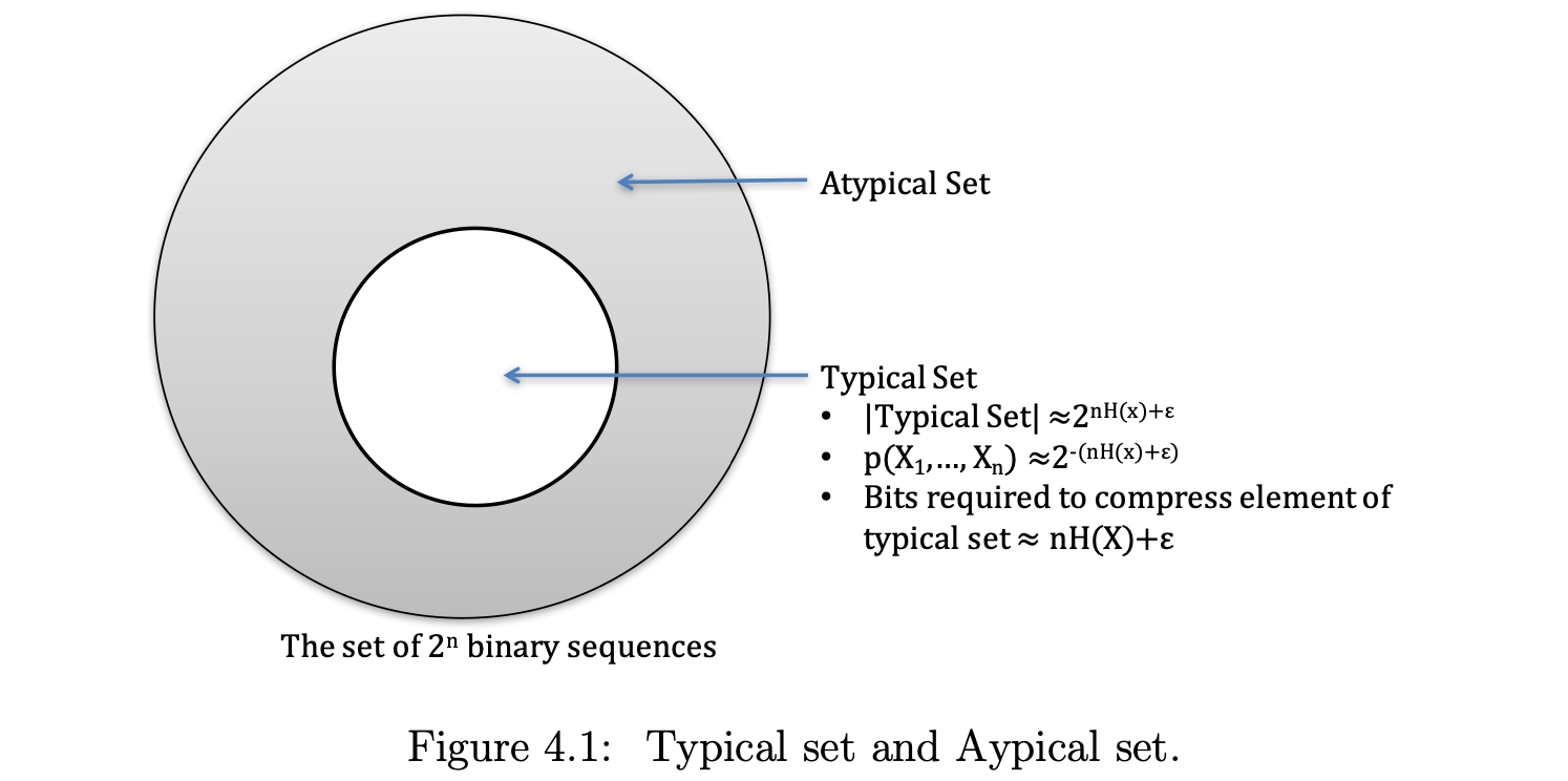
Note: the notation \(p(X_1, X_2, \cdots, X_n)\) in the above figure is denoted as \(p(X^n)\) is this post.
Theorem: Bound of \(\left|A_\epsilon^{(n)}\right|\)
Theorem: \(\forall \epsilon>0\) and \(n\) sufficiently large, \[ \begin{align} & \quad (1-\epsilon) \cdot 2^{n(H(X)-\epsilon)} \nonumber \\ \leq & \quad \left|A_\epsilon^{(n)}\right| \label{eq3} \\ \leq & \quad2^{n(H(u)+\epsilon)} \nonumber . \end{align} \]
Proof
Upper bound:
See following equation: \[ \begin{align} 1 & \geq P\left(X^n \in A_\epsilon^{(n)}\right) \label{eq3.1} \\ & \geq \sum_{X^n \in A_\epsilon^{(n)}} 2^{-n(H(X)+\epsilon)} \label{eq3.2} \\ & =2^{-n(H(X)+\epsilon)} \cdot\left|A_\epsilon^{(n)}\right| \label{eq3.3} \nonumber. \end{align} \]
\(\eqref{eq3.1}\) is due to the non-negativity of any probability.
\(\eqref{eq3.2}\) is due to \(\eqref{eq2.3}\).
According to \(\eqref{eq3.3}\), we have \[ \left|A_\epsilon^{(n)}\right| \leq 2^{n(H(X)+\epsilon)}. \]
Lower bound:
See following equation: \[ \begin{align} 1-\epsilon & \leq P\left(X^n \in A_\epsilon^{(n)}\right) \label{eq3.4} \\ & \leq \sum_{u^n \in A_\epsilon^{(n)}} 2^{-n(H(X)-\epsilon)} \nonumber \\ & =2^{-n(H(X)-\epsilon)} \cdot\left|A_\epsilon^{(n)}\right| \label{eq3.5}. \end{align} \]
The starting equation \(\eqref{eq3.4}\) in the lower bound proof is a consequence of Theorem: \(P\left(X^n \in A_\epsilon^{(n)}\right) \approx 1\).
Since \(P\left(X^n \in A_\epsilon^{(n)}\right) \stackrel{n \rightarrow \infty}{\longrightarrow} 1\), we can choose a sufficiently large \(n\) such that \(P\left(X^n \in A_\epsilon^{(n)}\right) \geq 1-\epsilon, \quad \forall \epsilon>0\).
According to \(\eqref{eq3.5}\), we have \[ \left|A_\epsilon^{(n)}\right| \geq(1-\epsilon) \cdot 2^{n(H(X)-\epsilon)}. \]
Theorem: \(A_\epsilon^{(n)}\) is an exponentially smaller than \(\mathcal{X}^n\)
The space of all possible source sequences \(\mathcal{X}^n\) has exponential size \(\left|\mathcal{X}^n\right|=r^n\), and the \(\epsilon\)-typical set \(A_\epsilon^{(n)}\) comprises a tiny fraction of \(\mathcal{X}^n\) with size \(\left|A_\epsilon^{(n)}\right| \approx 2^{n H(X)}\).
In fact, \(A_\epsilon^{(n)}\) is an exponentially smaller than \(\mathcal{X}^n\), as indicated by the ratio of their sizes, except when \(\mathrm{X}\) is uniformly distributed. \[ \begin{align} \frac{\left|A_\epsilon^{(n)}\right|}{\left|\mathcal{X}^n\right|} \nonumber & \approx \frac{2^{n H(X)}}{r^n} \nonumber\\ & = \frac{2^{n H(X)}}{2^{n \log r}} \nonumber\\ & =2^{-n(\log r-H(X))} \nonumber. \end{align} \]
Despite the small size of \(A_\epsilon^{(n)}\), the probabilistic mass in \(\mathcal{X}^n\) is almost entirely concentrated in \(A_\epsilon^{(n)}\). The forthcoming theorem illustrates the point that any subset of \(\mathcal{X}^n\) that's smaller than \(A_\epsilon^{(n)}\) fails to capture almost all of its probabilistic mass. Thus, \(A_\epsilon^{(n)}\) is minimal.
Theorem: \(A_\epsilon^{(n)}\) is minimal
Theorem: Fix \(\delta>0\) and \(B_{\delta}^{(n)} \subseteq \mathcal{X}^n\) such that \(\left|B_{\delta}^{(n)}\right| \leq 2^{n(H(X)-\delta)}\). Then \[ \begin{equation} \label{eq5} \lim _{n \rightarrow \infty} P\left(X^n \in B_{\delta}^{(n)}\right)=0 \end{equation} \]
Proof
$$ \[\begin{align} & \quad P\left(X^n \in B_{\delta}^{(n)}\right) \nonumber \\ & =P\left(X^n \in B_{\delta}^{(n)} \cap A_\epsilon^{(n)}\right)+P\left(X^n \in B_{\delta}^{(n)} \cap \complement A_\epsilon^{(n)}\right) \label{eq5.1} \\ & \leq P\left(X^n \in B_{\delta}^{(n)} \cap A_\epsilon^{(n)}\right)+P\left(X^n \notin A_\epsilon^{(n)}\right) \label{eq5.2} \\ & =\sum_{X^n \in B_{\delta}^{(n)} \cap A_\epsilon^{(n)}} P\left(X^n\right)+P\left(X^n \notin A_\epsilon^{(n)}\right) \label{eq5.3} \\ & \leq \sum_{u^n \in B_{\delta}^{(n)} \cap A_\epsilon^{(n)}} 2^{-n(H(X)-\epsilon)}+P\left(X^n \notin A_\epsilon^{(n)}\right) \label{eq5.4} \\ & =\left|B_{\delta}^{(n)} \cap A_\epsilon^{(n)}\right| \cdot 2^{-n(H(X)-\epsilon)}+P\left(X^n \notin A_\epsilon^{(n)}\right) \label{eq5.5} \\ & \leq \left|B_{\delta}^{(n)}\right| \cdot 2^{-n(H(X)-\epsilon)}+P\left(X^n \notin A_\epsilon^{(n)}\right) \label{eq5.6} \\ & \leq 2^{n(H(X)-\delta)} \cdot 2^{-n(H(X)-\epsilon)}+P\left(X^n \notin A_\epsilon^{(n)}\right) \label{eq5.7} \\ & =\underbrace{2^{-n(\delta-\epsilon)}}_{\rightarrow 0 \text { as } n \rightarrow \infty}+\underbrace{P\left(X^n \notin A_\epsilon^{(n)}\right)}_{\rightarrow 0 \text { as } n \rightarrow \infty} \label{eq5.8} \end{align}\] $$
Explaination:
\(\eqref{eq5.1}\) is derived from a basic theorem of sets. That is, given arbitary sets \(B, A\), \[ \begin{equation} \label{eq5.9} B = (B \cap A) \cup (B \cup \complement A) \end{equation} \] The proof is in appendix.
Then, we have \[ B_{\delta}^{(n)} = (B_{\delta}^{(n)} \cap A_\epsilon^{(n)}) \cup (B_{\delta}^{(n)} \cap (\complement A_\epsilon^{(n)}) \]
\(\eqref{eq5.2}\) is because given arbitary sets \(A, B\), \[ A \cap B \subseteq A \] Then we have \[ B_{\delta}^{(n)} \cap \complement A_\epsilon^{(n)} \subseteq \complement A_\epsilon^{(n)} \] And we also know \(X^n \in \complement A_\epsilon^{(n)} = X^n \notin A_\epsilon^{(n)}\).
Then \[ P(X^n \in B_{\delta}^{(n)} \cap \complement A_\epsilon^{(n)} ) \le P (X^n \notin A_\epsilon^{(n)}) \]
\(\eqref{eq5.3}\) is because all \(X^n\) are independent? //TODO
\(\eqref{eq5.4}\) is due to \(\eqref{eq2.3}\).
\(\eqref{eq5.5}\) is a common computation.
\(\eqref{eq5.6}\) is because given arbitary sets \(A, B\), \[ A \cap B \subseteq A \] Then we have \[ (B_{\delta}^{(n)} \cap A_\epsilon^{(n)}) \subseteq B_{\delta}^{(n)} \]
\(\eqref{eq5.7}\) is due to the prerequisite \(\left|B_{\delta}^{(n)}\right| \leq 2^{n(H(X)-\delta)}\).
The limit in \(\eqref{eq5.7}\) is easy to understand. Because \[ \forall \epsilon>0, P\left(X^n \in A_\epsilon^{(n)}\right) \stackrel{n \rightarrow \infty}{\longrightarrow} 1 \] Then we have \[ \forall \epsilon>0, P\left(X^n \notin A_\epsilon^{(n)}\right) \stackrel{n \rightarrow \infty}{\longrightarrow} 0 \]
From the theorems proven above, we understand \(A_\epsilon^{(n)}\) as a subset of \(\mathcal{X}^n\) that most efficiently contains virtually all of the source sequences that can be drawn from \(\mathcal{X}^n\). The following section confirms the intuition that, when developing a scheme which encodes sequences from \(\mathcal{X}^n\), we should focus our efforts towards the sequences that lie in \(A_\epsilon^{(n)}\).
Appendix
Proof of \(\eqref{eq5.9}\) "Given arbitary sets \(A, B\), \(B = (B \cap A) \cup (B \cup \complement A)\)":
Inclusion (\(\subseteq\)):
Let \(x\) be an arbitrary element in \(B\). We want to show that \(x\) is also in the right-hand side of the equation.
- If \(x∈B \cap A\): \(x\) is in the intersection of \(B\) and \(A\).
- If \(x∈ B \cap \complement A\): \(x\) is in the intersection of \(B\) and the complement of \(A\).
Therefore, \(B \subseteq (B \cap A) \cup (B \cup \complement A)\).
Inclusion (\(\supseteq\)):
Let \(y\) be an arbitrary element in \((B \cap A) \cup (B \cup \complement A)\). We want to show that \(y\) is also in \(B\).
- If \(y \in B \cap A\): \(y\) is in the intersection of \(B\) and \(A\), so yy is in \(B\).
- If \(y \in B \cap \complement A\): \(y\) is in the intersection of \(B\) and the complement of \(A\), so \(y\) is in \(B\).
Since \(y\) could be in either \(B \cap A\) or \(B \cap \complement A\), we can conclude that \(y\) is in \(B\).
Therefore, \((B \cap A) \cup (B \cup \complement A) \subseteq B\).
Combining both inclusions, we have \(B = (B \cap A) \cup (B \cup \complement A)\).