Shannon Entropy
Sources:
- Elements of Information Theory
- An Introduction to Single-User Information Theory
Entropy
Entropy is a fundamental concept in information theory. It's a measure of the average uncertainty in the random variable. It is the number of bits on average required to describe the random variable.
Note:
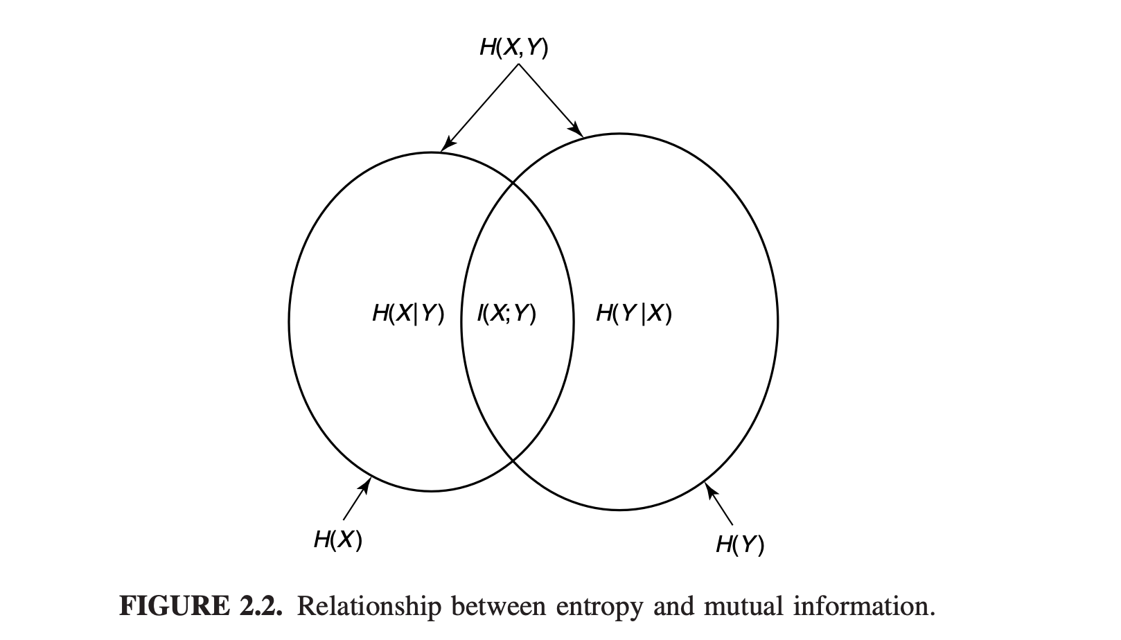
joint entropy \(H(X,Y)\) 可想象成把两个区域并联, 即 \(H(X)\)的部分 加上 \(H(Y)\)中挖掉\(H(X)\)的部分. \[ H(X,Y) = H(X) + H(X|Y) . \]
conditional entropy \(H(Y|X)\) 可想象成把\(H(Y)\)的区域挖掉 和\(H(X)\)相关 的部分, 也就是所谓的Theorem: Conditioning reduces entropy). \[ H(Y|X) = H(Y) - I(X;Y) . \]
mutual information \(I(X:Y)\) 可想象成\(H(X)\) 和 \(H(Y)\) 的交集: \[ I(X;Y) = H(X) - H(X|Y) = H(Y) - H(Y|X) . \]
Shannon Entropy
Definition: The entropy of a discrete random variable \(X\) with pmf \(P_X(\cdot)\) is denoted by \(H(X)\) or \(H\left(P_X\right)\) and defined by \[ H_b(X):=-\sum_{x \in \mathcal{X}} P_X(x) \cdot \log _2 P_X(x) \quad \text { (bits) } \] The formula for information entropy was introduced by Claude E. Shannon in his 1948 paper "A Mathematical Theory of Communication".
- Label-invariance: Entropy is label-invariant, meaning that it depends only on the probability distribution and not on the actual values that the random variable \(X\).
- E.g.,\(H(5X) = H(X)\) because \(5X\) and \(X\) share the same probability distribution.
- Notably, \(H (X)\) is itself a random variable, because \(X\) is a random variable.
- Symbol convention:
- \(\log\) is assumed to be \(\log_2\) unless otherwise indicated.
- (在 \(\log\)函数 底为2时)Entropy的单位是bit.
- \(H(X)\)的下标取决于使用的\(\log\)函数的底. 因此\(H(X), H_2(X), H_b(X)\)是相同的(\(b\)代表二进制的比特). 如果 \(\log\)函数 使用其它底, 设为\(a\), 那么必须清楚地在文中说明: \(H_a(X) = \sum_x p(x) \log _a \frac{1}{p(x)}\).
Properties
Lemma1: \(H(X) \geq 0\).
Proof:
\(\quad 0 \leq p(x) \leq 1\) implies that \(\log \frac{1}{p(x)} \geq 0\).
Lemma2: \(H_b(X)=\left(\log _b a\right) H_a(X)\).
Proof:
Since \(\log_a b = \frac{\log_c b}{\log_c a}\).
Then \(\log _b p=\log _b a \log _a p\).
So \(H_2(X) = \sum_x p(x) \log _2 \frac{1}{p(x)} = \log_2 a . \sum_x p(x) \log _a \frac{1}{p(x)} = ( \log_2 a)H_a(X)\).
Example: For Bernoulli Distribution
Here we discuss the entropy of random variable \(X\) if \(X \sim \text{Bern}(p)\) (Bernoulli distribution).
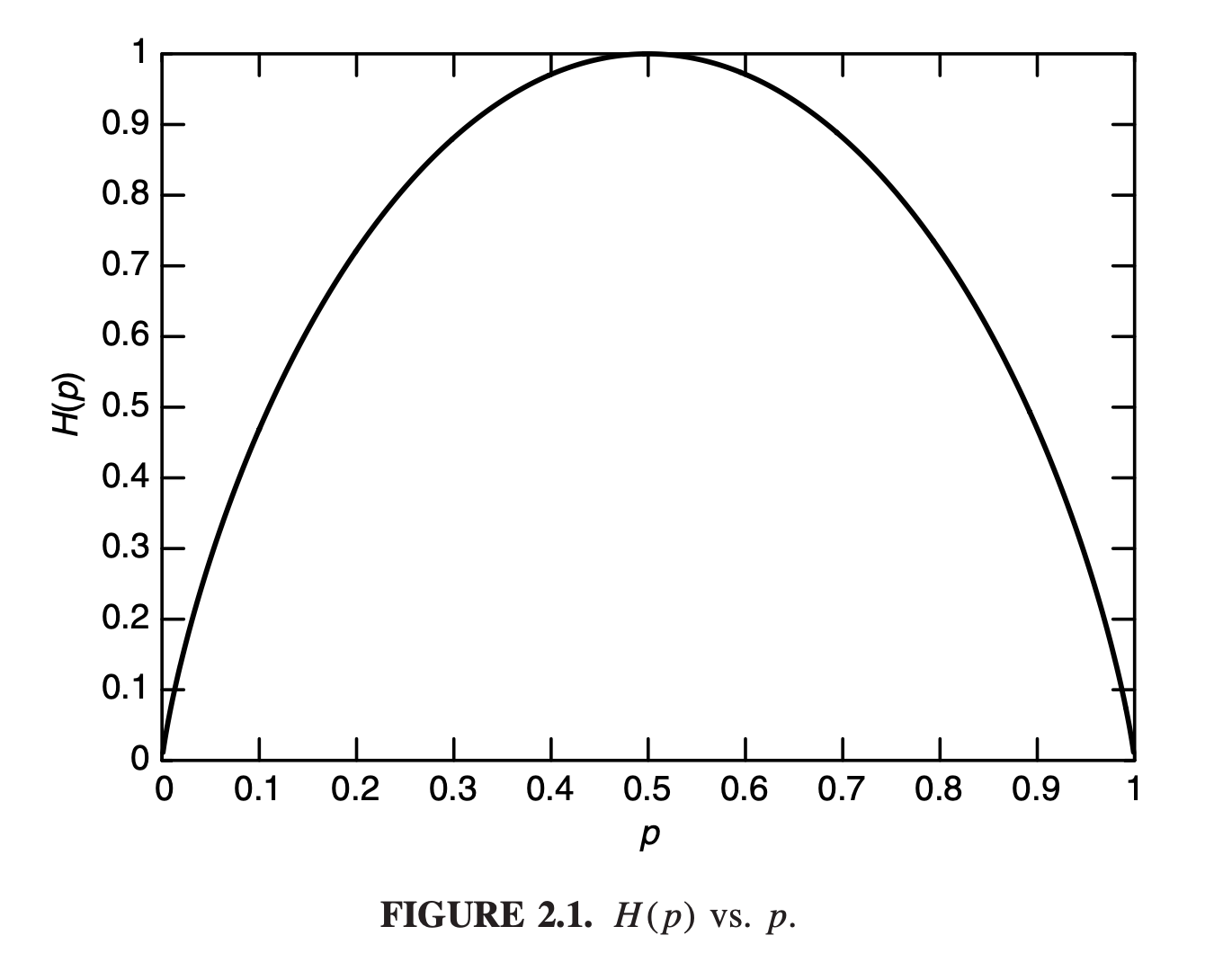
In this scenario, \(X \in \{0,1\}\) and \(\operatorname{Pr}[X=0]=p\), so we can compute the entropy of the distribution (dropping the base 2 ) as \[ H(X)=\mathbb{E}\left[\log \frac{1}{p(X)}\right]=p \log \frac{1}{p}+(1-p) \log \frac{1}{1-p} . \] we get the curve in figure 2.1 which reaches a maximum of 1 when \(p=0.5\).
我们可以以抛硬币为例, 对于一个正常的硬币, 其每面的概率都是0.5, 令\(X\)为硬币朝上那面的值, \(X \in X \in \{0,1\}\), \(p = 0.5\).
此时有 \(H(X)=0.5(1)+0.5(1)=1\).
What about for a coin that almost always lands tails \((X=0)\), with \(p=0.999\) ?
With this heavily-biased coin, we get \(H(X)=0.999 \log \frac{1}{0.999}+0.001 \log \frac{1}{0.001} \approx 0.011\).
From this example, we can see that we gain more information from more surprising events (i.e., \(\log \frac{1}{p(x)} \uparrow\) as \(p(x) \downarrow\) ), but they also happen less often.
Example: Uniform Distribution
For a discrete random variable \(X\) with a uniform distribution over \(n\) outcomes, each with probability \(P(X=x_i)=\frac{1}{n}\), the entropy \(H(X)\) is calculated as follows: \[ \begin{aligned} H(X) &=−\sum_{i=1}^{n}P(X=x_i) \log P(X=x_i) \\ &= n \cdot \frac{1}{n} \cdot \log \frac{1}{\frac{1}{n}} \\ &= 1 \cdot \log n \\ &= \log n \end{aligned} \]
Joint Entropy
There is nothing really new in this definition because \((X,Y)\) can be considered to be a single vector-valued random variable.
Definition: The joint entropy \(H(X, Y)\) of random variables \((X, Y)\) is defined by \[ \begin{aligned} H(X, Y) & :=-\sum_{(x, y) \in \mathcal{X} \times \mathcal{Y}} P_{X, Y}(x, y) \cdot \log _2 P_{X, Y}(x, y) \\ & = \mathbb E\left[\log _2 \frac {1} {P_{X, Y}(X, Y)} \right] . \end{aligned} \]
The conditional entropy can be similarly defined as follows.
Conditional Entropy
Definition: Given two jointly distributed random variables \(X\) and \(Y\), the conditional entropy \(H(Y \mid X)\) of \(Y\) given \(X\) is defined by \[ H(Y \mid X):=\sum_{x \in \mathcal{X}} P_X(x)\left(-\sum_{y \in \mathcal{Y}} P_{Y \mid X}(y \mid x) \cdot \log _2 P_{Y \mid X}(y \mid x)\right), \] where \(P_{Y \mid X}(\cdot \mid \cdot)\) is the conditional pmf of \(Y\) given \(X\). This equation can be written into three different but equivalent forms: \[ \begin{aligned} H(Y \mid X) & =-\sum_{(x, y) \in \mathcal{X} \times \mathcal{Y}} P_{X, Y}(x, y) \cdot \log _2 P_{Y \mid X}(y \mid x) \\ & =\mathbb E\left[\log _2 \frac {1} {P_{Y \mid X}(Y \mid X)} \right] \\ & =\sum_{x \in \mathcal{X}} P_X(x) \cdot H(Y \mid X=x) \end{aligned} \] where \(H(Y \mid X=x):=-\sum_{y \in \mathcal{Y}} P_{Y \mid X}(y \mid x) \log _2 P_{Y \mid X}(y \mid x)\).
\(\sum_{x, y} p(x, y)\)也可写作\(\sum_{x \in \mathcal X} \sum_{y \in \mathcal Y} p(x, y)\).
The first line equals \(-\sum_{(x, y) \in \mathcal{X} \times \mathcal{Y}} P_Y(y) \cdot P_{Y|X}(y|x) \cdot \log _2 P_{Y \mid X}(y \mid x)\), and \(\sum_{x,y} \triangleq \sum_x \sum_y\). We can extract the \(\sum_x\) outside, resulting in \[ -\sum_{x \in \mathcal{X}} P_X(x) \sum_{y \in \mathcal Y} P(y|x) \cdot \log _2 P_{Y \mid X}(y \mid x) = \sum_{x \in \mathcal{X}} P_X(x) \cdot H(Y \mid X=x) . \]
The probability distributions for the expectation and in the function itself are not the same! If you are unhappy with that, just remember that for any arbitrary function, \(\mathbb{E}[f(X, Y)]=\sum_{x, y} p(x, y) f(x, y)\), and in this case, that arbitrary function is \(\log \frac{1}{p(y \mid x)}\).
The relationship between joint entropy and conditional entropy is exhibited by the fact that the entropy of a pair of random variables is the entropy of one plus the conditional entropy of the other.
Chain Rule for Entropy(2 Variables)
Note: 本文仅探讨2-3个随机变量的变量的entropy的Chain Rule, 更general的chain rule的探讨请参见Chain Rules for Entropy, Relative Entropy and Mutual Information.
\[ \begin{equation} \label{eq4} H(X, Y)=H(X)+H(Y \mid X) . \end{equation} \]
Proof: Short
简短证明, 只使用数学期望.
\[ \begin{aligned} H(X, Y) & =\mathbb{E}\left[\log \frac{1}{p(x) p(y \mid x)}\right] \\ & =\mathbb{E}\left[\log \frac{1}{p(x)}\right]+\mathbb{E}\left[\log \frac{1}{p(y \mid x)}\right] \\ H(X, Y) & =H(X)+H(Y \mid X) \end{aligned} \]
Proof: Long
复杂证明, 从\(\log\)函数出发.
By definition, we have \[ \begin{aligned} H(X, Y) & =-\sum_{x \in \mathcal{X}} \sum_{y \in \mathcal{Y}} p(x, y) \log p(x, y) \\ \end{aligned} \] According to Bayes' theorem \(\log p(x, y) = \log p(x) \log p(y | x)\), \[ -\sum_{x \in \mathcal{X}} \sum_{y \in \mathcal{Y}} p(x, y) \log p(x, y) =-\sum_{x \in \mathcal{X}} \sum_{y \in \mathcal{Y}} p(x, y) \log [p(x) p(y \mid x)] \]
Since \(\log_b ac = \log_b a + \log_b c\) \[ -\sum_{x \in \mathcal{X}} \sum_{y \in \mathcal{Y}} p(x, y) \log [p(x) p(y \mid x)] = -\sum_{x \in \mathcal{X}} \sum_{y \in \mathcal{Y}} p(x, y) \log p(x)-\sum_{x \in \mathcal{X}} \sum_{y \in \mathcal{Y}} p(x, y) \log p(y \mid x) \]
Because \(p(x)\) is a marginal probability, \(p(x) = \sum_{y \in \mathcal{Y}} p(x, y)\). We have
\[ -\sum_{x \in \mathcal{X}} \sum_{y \in \mathcal{Y}} p(x, y) \log p(x)-\sum_{x \in \mathcal{X}} \sum_{y \in \mathcal{Y}} p(x, y) \log p(y \mid x) \\=-\sum_{x \in \mathcal{X}} p(x) \log p(x)-\sum_{x \in \mathcal{X}} \sum_{y \in \mathcal{Y}} p(x, y) \log p(y \mid x) \] By definition: \[ -\sum_{x \in \mathcal{X}} p(x) \log p(x)-\sum_{x \in \mathcal{X}} \sum_{y \in \mathcal{Y}} p(x, y) \log p(y \mid x) =H(X)+H(Y \mid X) \] Q.E.D.
Theorem: Function reduces entropy
Let \(X\) be a discrete random variable. That the entropy of a function of \(X\) is less than or equal to the entropy of \(X\) by justifying the following steps: \[ \begin{aligned} H(X, g(X)) & \stackrel{(a)}{=} H(X)+H(g(X) \mid X) \\ & \stackrel{(b)}{=} H(X) ; \\ H(X, g(X)) & \stackrel{(c)}{=} H(g(X))+H(X \mid g(X)) \\ & \stackrel{(d)}{\geq} H(g(X)) . \end{aligned} \]
Thus \(H(g(X)) \leq H(X)\). Explanation:
\(H(X, g(X))=H(X)+H(g(X) \mid X)\) by the chain rule for entropies.
\(H(g(X) \mid X)=0\) is because: Since for any particular value of \(X, g(X)\) is fixed, then \(p(g(X)=g(x)|X=x) = 1\). By definition of conditional entropy: \[ H(X,g(X)) = -\sum_{(x, g(x)) } p(x, g(x)) \cdot \log _2 p[g(x) \mid x] = -\sum_{(x, g(x)) } p(x, g(x)) \cdot 0 = 0 \] Meanwhile, if \(H(Y|X) = 0\), we can also say \(Y\) is a function(or injection) of \(X\).
\(H(X, g(X))=H(g(X))+H(X \mid g(X))\) again by the chain rule.
\(H(X \mid g(X)) \geq 0\), with equality iff \(X\) is a function of \(g(X)\), i.e., \(g(\cdot)\) is one-to-one. Hence \(H(X, g(X)) \geq\) \(H(g(X))\).
Combining (1)-(4), we obtain \(H(X) \geq H(g(X))\).
Properties of Joint Entropy and Conditional Entropy
\(H(Y|X) \le H(Y)\)
\(H(Y|X) \le H(Y)\)( see ->proof ) with equality holding iff \(X\) and \(Y\) are independent.
Entropy is additive for independent r.v.
Entropy is additive for independent random variables; i.e., \[ \begin{aligned} H\left(X, Y\right) & =\mathbb{E}\left[\log \frac{1}{p\left(X,Y\right)}\right] \\ & =\mathbb{E}\left[\log \frac{1}{p\left(X\right) p\left(Y\right)}\right] \\ & =\mathbb{E}\left[\log \frac{1}{p\left(X\right)}\right]+\mathbb{E}\left[\log \frac{1}{p\left(Y\right)}\right] \\ & =H\left(X\right)+H\left(Y\right) . \end{aligned} \]
- The 2nd line holds since \(X,Y\) are independent.
If \(X\) and \(Y\) are not independent, we can use chain rule to compute \(H(X,Y)\).
Conditional entropy is lower additive
Conditional entropy is lower additive; i.e., \[ H\left(X_1, X_2 \mid Y_1, Y_2\right) \leq H\left(X_1 \mid Y_1\right)+H\left(X_2 \mid Y_2\right) . \] Equality holds iff \[ P_{X_1, X_2 \mid Y_1, Y_2}\left(x_1, x_2 \mid y_1, y_2\right)=P_{X_1 \mid Y_1}\left(x_1 \mid y_1\right) P_{X_2 \mid Y_2}\left(x_2 \mid y_2\right) \] for all \(x_1, x_2, y_1\) and \(y_2\).
Proof: Using the chain rule for conditional entropy and the fact that conditioning reduces entropy, we can write \[ \begin{aligned} H\left(X_1, X_2 \mid Y_1, Y_2\right) & =H\left(X_1 \mid Y_1, Y_2\right)+H\left(X_2 \mid X_1, Y_1, Y_2\right) \\ & \leq H\left(X_1 \mid Y_1, Y_2\right)+H\left(X_2 \mid Y_1, Y_2\right) \\ & \leq H\left(X_1 \mid Y_1\right)+H\left(X_2 \mid Y_2\right) \end{aligned} \]
For the 2nd line, equality holds iff \(X_1\) and \(X_2\) are conditionally independent given \(\left(Y_1, Y_2\right)\) : \(P_{X_1, X_2 \mid Y_1, Y_2}\left(x_1, x_2 \mid y_1, y_2\right)=P_{X_1 \mid Y_1, Y_2}\left(x_1 \mid y_1, y_2\right) P_{X_2 \mid Y_1, Y_2}\left(x_2 \mid y_1, y_2\right)\).
For the 3rd line, equality holds iff \(X_1\) is conditionally independent of \(Y_2\) given \(Y_1\) (i.e., \(P_{X_1 \mid Y_1, Y_2}\left(x_1 \mid y_1, y_2\right)=\) \(P_{X_1 \mid Y_1}\left(x_1 \mid y_1\right)\) ), and \(X_2\) is conditionally independent of \(Y_1\) given \(Y_2\) (i.e., \(P_{X_2 \mid Y_1, Y_2}\left(x_2 \mid y_1\right.\), \(\left.\left.y_2\right)=P_{X_2 \mid Y_2}\left(x_2 \mid y_2\right)\right)\).
Hence, the desired equality condition of the lemma is obtained.
Others
Suppose that \(X\) is a random variable whose entropy \(H(X)\) is \(k\) bits. Suppose that \(Y(X)\) is a deterministic function that takes on a different value for each value of \(X\).
- \(H(Y ) = k \quad \text{bits}\) also.
- The conditional entropy of Y given X: \(H(Y|X) = 0\) because of determinism.
- The conditional entropy of X given Y : \(H(X|Y) = 0\) also.
- The joint entropy \(H(X, Y) = H(X) + H(Y|X) = k \quad \text{bits}\).
Suppose now that the deterministic function \(Y(X)\) is not invertible; in other words, different values of \(X\) may correspond to the same value of \(Y(X)\). In that case,
- The new distribution of \(Y\) has lost entropy and so \(H(Y) < k \quad \text{bits}\).
- Now knowledge of Y no longer determines \(X\), and so the conditional entropy \(H(X|Y)\) is no longer zero: \(H(X|Y) > 0\).