Jensen’s Inequality
Sources:
- Elements of Information Theory
- EE 376A: Information Theory - Stanford University
Convexity
Convexity underlies many of the basic properties of information-theoretic quantities such as entropy and mutual information.
Definition: A function \(f(x)\) is said to be convex(凸函数) over an interval \((a, b)\) if for every \(x_1, x_2 \in(a, b)\) and \(0 \leq \lambda \leq 1\), \[ \begin{equation} \label{eq1} f\left(\lambda x_1+(1-\lambda) x_2\right) \leq \lambda f\left(x_1\right)+(1-\lambda) f\left(x_2\right) . \end{equation} \] A function \(f\) is said to be strictly convex if equality holds only if \(\lambda=0\) or \(\lambda=1\).
Note: A function \(f\) is concave(凹函数) if \(-f\) is convex.
A function is convex if it always lies below any chord. A function is concave if it always lies above any chord.
Examples
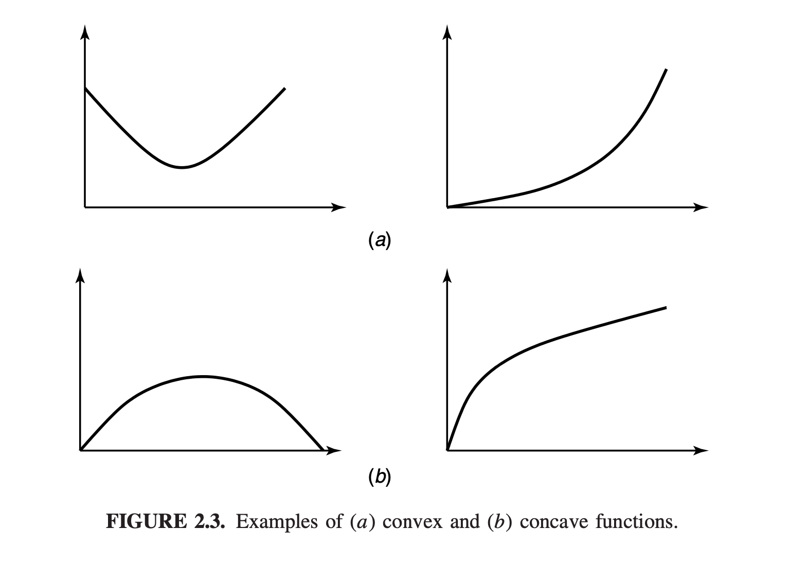
- Examples of convex functions: \(x^2,|x|, e^x, x \log x\) (for \(x \geq\) 0 ), and so on.
- Examples of concave functions: \(\log x\) and \(\sqrt{x}\) for \(x \geq 0\).
- Note: linear functions \(a x+b\) are both convex and concave.
Theorem 1
If the function f has a second derivative that is non- negative (positive) over an interval, the function is convex (strictly convex) over that interval.
Proof: We use the Taylor series expansion(泰勒展开) of the function around \(x_0\) : \[ f(x)=f\left(x_0\right)+f^{\prime}\left(x_0\right)\left(x-x_0\right)+\frac{f^{\prime \prime}\left(x^*\right)}{2}\left(x-x_0\right)^2, \] where \(x^*\) lies between \(x_0\) and \(x\).
By hypothesis, \(f^{\prime \prime}\left(x^*\right) \geq 0\), and thus the last term is nonnegative for all \(x\). So \[ f(x) \ge f(x) - \frac{f^{\prime \prime}\left(x^*\right)}{2}\left(x-x_0\right)^2 = f\left(x_0\right)+f^{\prime}\left(x_0\right)\left(x-x_0)\right). \]
We let \(x_0=\lambda x_1+(1-\lambda) x_2\) and take \(x=x_1\), to obtain \[ \begin{equation} \label{eq1.1} f\left(x_1\right) \geq f\left(x_0\right)+f^{\prime}\left(x_0\right)\left((1-\lambda)\left(x_1-x_2\right)\right). \end{equation} \]
Similarly, taking \(x=x_2\), we obtain \[ \begin{equation} \label{eq1.2} f\left(x_2\right) \geq f\left(x_0\right)+f^{\prime}\left(x_0\right)\left(\lambda\left(x_2-x_1\right)\right) . \end{equation} \] Multiplying \(\eqref{eq1.1}\) by \(\lambda\) and \(\eqref{eq1.2}\) by \(1-\lambda\) and adding, we obtain \(\eqref{eq1}\). The proof for strict convexity proceeds along the same lines.
Theorem 1 allows us immediately to verify the strict convexity of \(x^2, e^x\), and \(x \log x\) for \(x \geq 0\), and the strict concavity of \(\log x\) and \(\sqrt{x}\) for \(x \geq 0\).
Let \(E\) denote expectation. Thus, \(E X=\sum_{x \in \mathcal{X}} p(x) x\) in the discrete case and \(E X=\int x f(x) d x\) in the continuous case.
Jensen’s Inequality
Definition: If \(f\) is a convex function and \(X\) is a random variable, the Jensen’s inequality is defined as \[ \begin{equation} \label{eq2} E f(X) \geq f(E X) . \end{equation} \] Moreover, if \(f\) is strictly convex, the equality in \(\eqref{eq2}\) implies that \(X=E X\) with probability 1 (i.e., \(X\) is a constant).
Proof
We prove this for discrete distributions by induction on the number of mass points. The proof of conditions for equality when \(f\) is strictly convex is left to the reader. For a two-mass-point distribution, the inequality becomes \[ p_1 f\left(x_1\right)+p_2 f\left(x_2\right) \geq f\left(p_1 x_1+p_2 x_2\right), \] which follows directly from the definition of convex functions. Suppose that the theorem is true for distributions with \(k-1\) mass points. Then writing \(p_i^{\prime}=p_i /\left(1-p_k\right)\) for \(i=1,2, \ldots, k-1\), we have
\[ \begin{aligned} \sum_{i=1}^k p_i f\left(x_i\right) & =p_k f\left(x_k\right)+\left(1-p_k\right) \sum_{i=1}^{k-1} p_i^{\prime} f\left(x_i\right) \\ & \geq p_k f\left(x_k\right)+\left(1-p_k\right) f\left(\sum_{i=1}^{k-1} p_i^{\prime} x_i\right) \\ & \geq f\left(p_k x_k+\left(1-p_k\right) \sum_{i=1}^{k-1} p_i^{\prime} x_i\right) \\ & =f\left(\sum_{i=1}^k p_i x_i\right) \end{aligned} \] where the first inequality follows from the induction hypothesis and the second follows from the definition of convexity.
The proof can be extended to continuous distributions by continuity arguments.
We now use these results to prove some of the properties of entropy and relative entropy. The following theorem is of fundamental importance.
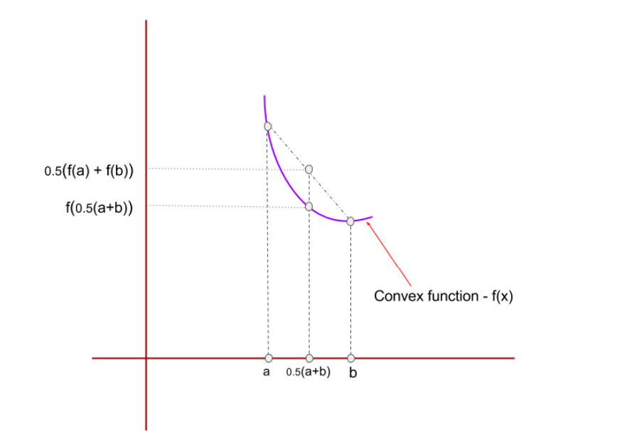
Example
Consider a uniform random variable \(X\) defined on set \(\{a, b\}\) and a convex function \(f\) as shown in Figure 3.
By Jensen’s inequality, \(0.5 f(a) + f(b) \ge f 0.5(a + b)\) , which can also be inferred from Figure 3.
Theorem: Information Inequality
Let \(p(x), q(x), x \in \mathcal{X}\), be two probability mass functions. Then \[ D(p \| q) \geq 0 \] with equality if and only if \(p(x)=q(x)\) for all \(x\). Proof: Let \(A=\{x | p(x)>0\}\) be the support set1 of \(p(x)\). Then \[ \begin{align} -D(p \| q) & =-\sum_{x \in A} p(x) \log \frac{p(x)}{q(x)} \nonumber \\ & =\sum_{x \in A} p(x) \log \frac{q(x)}{p(x)} \nonumber \\ & = \mathbb E_{x \in A}(\log \frac{q(x)}{p(x)}) \nonumber \\ & \leq \log \mathbb E_{x \in A}(\frac{q(x)}{p(x)}) \label{eq3.1}\\ & = \log \sum_{x \in A} p(x) \frac{q(x)}{p(x)} \nonumber\\ & =\log \sum_{x \in A} q(x) \nonumber \\ & \leq \log \sum_{x \in \mathcal{X}} q(x) \label{eq3.2} \\ & =\log 1 \nonumber \\ & =0 \nonumber \end{align} \] where \(\eqref{eq3.1}\) follows from Jensen’s inequality, because \(\log t\) is a strictly concave function of \(t\).
Also, since \(\log t\) is a strictly concave function of \(t\), we have equality in \(\eqref{eq3.1}\) if and only if \(\frac {q(x)}{p(x)}\) is constant everywhere [i.e., \(q(x)=c p(x)\) for all \(x\) ]. Thus, \(\sum_{x \in A} q(x)=\) \(c \sum_{x \in A} p(x)=c\).
We have equality in \(\eqref{eq3.2}\) only if \(\sum_{x \in A} q(x)=\sum_{x \in \mathcal{X}}\) \(q(x)=1\), which implies that \(c=1\). Hence, we have \(D(p \| q)=0\) if and only if \(p(x)=q(x)\) for all \(x\).
Note: 证明中必须要用到support set \(A=\{x | p(x)>0\}\), 这是因为证明时出现了\(\frac {q(x)}{p(x)}\), 我们必须满足\(p(x) > 0\).
Theorem: \(H(X) \leq \log |\mathcal{X}|\)
We now show that the uniform distribution over the range \(\mathcal{X}\) is the maximum entropy distribution over this range. It follows that any random variable with this range has an entropy no greater than \(\log |\mathcal{X}|\).
Theorem: \[ H(X) \leq \log |\mathcal{X}| \] where \(|\mathcal{X}|\) denotes the number of elements in the range of \(X\), with equality if and only \(X\) has a uniform distribution over \(\mathcal{X}\).
Proof: \(\quad\) Let \(u(x)=\frac{1}{|\mathcal{X}|}\) be the uniform probability mass function over \(\mathcal{X}\), and let \(p(x)\) be the probability mass function for \(X\). Then \[ D(p \| u)=\sum p(x) \log \frac{p(x)}{u(x)}=\log |\mathcal{X}|-H(X) . \] Hence by the nonnegativity of relative entropy, \[ 0 \leq D(p \| u)=\log |\mathcal{X}|-H(X) . \]
Theorem: Conditioning reduces entropy
Conditioning reduces entropy(Information can’t hurt): \[ H(X \mid Y) \leq H(X) \] with equality if and only if \(X\) and \(Y\) are independent.
Proof:
- We know that \(0 \leq I(X ; Y)\)2.
- Since \(I(X ; Y)=H(X)-H(X \mid Y)\).
- We have \(H(X \mid Y) \leq H(X)\)
Intuitively, the theorem says that knowing another random variable \(Y\) can only reduce the uncertainty in \(X\).
Note that this is true only on the average. Specifically, \(H(X \mid Y=y)\) may be greater than or less than or equal to \(H(X)\), but on the average \(H(X \mid Y)=\sum_y p(y) H(X \mid Y=y) \leq\) \(H(X)\). For example, in a court case, specific new evidence might increase uncertainty, but on the average evidence decreases uncertainty.
For multiple condions
This theorem can be extended to multiple condions. Given random variables \(X_1, X_2, \cdots, X_n\), \[ H(X_1|X_2,X_3,\cdots,X_n) \le H(X_1|X_3,\cdots,X_n) . \] Proof:
- We know that \(0 \leq I(X_1|X_3,\cdots,X_n; X_2)\).
- Note that the conditional entropy of \(X|Y\) given observation \(Z\) is \(H(X | Y, Z)\). so \(I(X_1|X_3,\cdots,X_n; X_2)=H(X_1|X_3,\cdots,X_n)-H(X_1|X_2, X_3,\cdots,X_n)\).
- We have \(H(X_1|X_3,\cdots,X_n) \leq H(X_1|X_2, X_3,\cdots,X_n)\).
Example
Let \((X, Y)\) have the following joint distribution:
| Y\X | x=1 | x=2 |
|---|---|---|
| Y=1 | 0 | 3/4 |
| Y=2 | 1/8 | 1/8 |
Then we have
- \(H(X)=H\left(\frac{1}{8}, \frac{7}{8}\right)=0.544\) bit,
- \(H(X \mid Y=1)=0 \quad\) bits,
- \(H(X \mid Y=2)=1\) bit.
We calculate \(H(X \mid Y)=\frac{3}{4} H(X \mid Y=1)+\frac{1}{4}\) \(H(X \mid Y=2)=0.25\) bit.
Thus, the uncertainty in \(X\) is:
- increased if \(Y=2\) is observed
- decreased if \(Y=1\) is observed
But uncertainty decreases on the average.
Theorem: Independence bound on entropy
Let \(X_1, X_2, \ldots, X_n\) be drawn according to \(p\left(x_1, x_2, \ldots, x_n\right)\). Then \[ H\left(X_1, X_2, \ldots, X_n\right) \leq \sum_{i=1}^n H\left(X_i\right) \] with equality if and only if the \(X_i\) are independent.
Proof:
By the chain rule for entropies, \[ H\left(X_1, X_2, \ldots, X_n\right) =\sum_{i=1}^n H\left(X_i \mid X_{i-1}, \ldots, X_1\right) \]
Then by theorem of Conditioning reduces entropy, \[ \forall \ {i \in1, \cdots,n}, \ H\left(X_i \mid X_{i-1}, \ldots, X_1\right) \le H(X_i) \]
Then we have \[ \begin{aligned} H\left(X_1, X_2, \ldots, X_n\right) & =\sum_{i=1}^n H\left(X_i \mid X_{i-1}, \ldots, X_1\right) \\ & \leq \sum_{i=1}^n H\left(X_i\right) \end{aligned} \] According to theorem of Conditioning reduces entropy, we have equality if and only if \(X_i\) is independent of \(X_{i-1}, \ldots, X_1\) for all \(i\) (i.e., if and only if the \(X_i\) ’s are independent).
Q.E.D.